Black Hole Spectra

Black hole spectra can be generated by combining a BlackHoles object with an EmissionModel, translating the physical properties of the blackhole(s) (e.g. mass, accretion_rate, etc.) to a spectral energy distribution.

These models are described in detail in the emission model docs. Here, we’ll use an instance of a UnifiedAGN model for demonstration purposes.

The following sections demonstrate the generation of combined spectra (which is the same for both parametric and particle BlackHoles) and per–particle spectra.

import numpy as np
from unyt import K, Mpc, Msun, deg, yr

from synthesizer import Grid
from synthesizer.emission_models import (
    AttenuatedEmission,
    DustEmission,
    UnifiedAGN,
)
from synthesizer.emission_models.attenuation import PowerLaw
from synthesizer.emission_models.dust.emission import Greybody
from synthesizer.parametric import BlackHole

# Get the NLR and BLR grids
nlr_grid = Grid("test_grid_agn-nlr", grid_dir="../../../tests/test_grid")
blr_grid = Grid("test_grid_agn-blr", grid_dir="../../../tests/test_grid")

uniagn = UnifiedAGN(
    nlr_grid,
    blr_grid,
    covering_fraction_nlr=0.1,
    covering_fraction_blr=0.1,
    torus_emission_model=Greybody(1000 * K, 1.5),
)

blackhole = BlackHole(
    mass=1e8 * Msun,
    inclination=60 * deg,
    accretion_rate=1 * Msun / yr,
    metallicity=0.01,
)

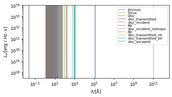
Integrated spectra

To generate integrated spectra we simply call the component’s get_spectra method. This method will populate the component’s spectra attribute with a dictionary containing Sed objects for each spectra in the EmissionModel. It will also return the spectra at the root of the EmissionModel.

# Get the spectra using a unified agn model (instantiated elsewhere)
spectra = blackhole.get_spectra(uniagn)

fig, ax = blackhole.plot_spectra(
    show=True, ylimits=(10**27.5, 10**34.0), figsize=(6, 4)
)

Including dust attenuation

We can also generate spectra including attenuation and emission from diffuse dust along the line of sight to the black hole. We do this by combining the UnifiedAGN model with models defining these attenuation and emission contributions.

First we define the emission models (for more details see the emission model docs).

tau_v = 0.5
dust_curve = PowerLaw(slope=-1.0)
dust_emission_model = Greybody(30 * K, 1.2)

# Define an emission model to attenuate the intrinsic AGN emission
att_model = AttenuatedEmission(
    dust_curve=dust_curve,
    apply_dust_to=uniagn,
    tau_v=tau_v,
    emitter="blackhole",
)

# And now include the dust emission
dust_model = DustEmission(
    dust_emission_model=dust_emission_model,
    dust_lum_intrinsic=uniagn,
    dust_lum_attenuated=att_model,
    emitter="blackhole",
)

We then follow the same process of calling get_spectra with the new model. The plot here shows luminosity rather than spectral energy density.

spectra = blackhole.get_spectra(dust_model)

fig, ax = blackhole.plot_spectra(quantity_to_plot="luminosity", figsize=(6, 4))

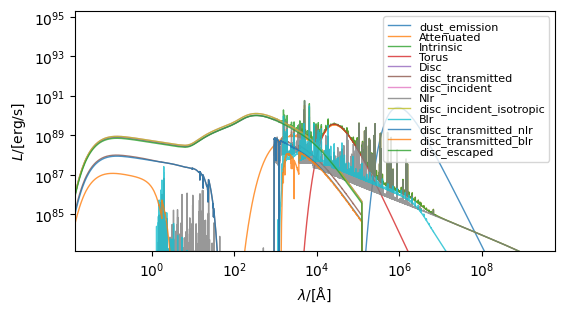
The spectra returned by get_spectra is the “dust_emission” spectra at the root of the emission model.

print(spectra)

+-------------------------------------------------------------------------------------------------+
|                                               SED                                               |
+---------------------------+---------------------------------------------------------------------+
| Attribute                 | Value                                                               |
+---------------------------+---------------------------------------------------------------------+
| redshift                  | 0                                                                   |
+---------------------------+---------------------------------------------------------------------+
| ndim                      | 1                                                                   |
+---------------------------+---------------------------------------------------------------------+
| shape                     | (9244,)                                                             |
+---------------------------+---------------------------------------------------------------------+
| lam (9244,)               | 1.30e-04 Å -> 2.99e+11 Å (Mean: 9.73e+09 Å)                         |
+---------------------------+---------------------------------------------------------------------+
| nu (9244,)                | 1.00e+07 Hz -> 2.31e+22 Hz (Mean: 8.51e+19 Hz)                      |
+---------------------------+---------------------------------------------------------------------+
| lnu (9244,)               | 0.00e+00 erg/(Hz*s) -> 1.36e+33 erg/(Hz*s) (Mean: 5.82e+31 erg)     |
+---------------------------+---------------------------------------------------------------------+
| bolometric_luminosity     | 4.537659655485052e+45 erg/s                                         |
+---------------------------+---------------------------------------------------------------------+
| bolometric_luminosity     | 4.537659655485052e+45 erg/s                                         |
+---------------------------+---------------------------------------------------------------------+
| energy (9244,)            | 4.14e-08 eV -> 9.56e+07 eV (Mean: 3.52e+05 eV)                      |
+---------------------------+---------------------------------------------------------------------+
| frequency (9244,)         | 1.00e+07 Hz -> 2.31e+22 Hz (Mean: 8.51e+19 Hz)                      |
+---------------------------+---------------------------------------------------------------------+
| llam (9244,)              | 0.00e+00 erg/(s*Å) -> 4.68e+39 erg/(s*Å) (Mean: 1.57e+38 erg/(s*Å)) |
+---------------------------+---------------------------------------------------------------------+
| luminosity (9244,)        | 0.00e+00 erg/s -> 3.96e+45 erg/s (Mean: 1.47e+44 erg/s)             |
+---------------------------+---------------------------------------------------------------------+
| luminosity_lambda (9244,) | 0.00e+00 erg/(s*Å) -> 4.68e+39 erg/(s*Å) (Mean: 1.57e+38 erg/(s*Å)) |
+---------------------------+---------------------------------------------------------------------+
| luminosity_nu (9244,)     | 0.00e+00 erg/(Hz*s) -> 1.36e+33 erg/(Hz*s) (Mean: 5.82e+31 erg)     |
+---------------------------+---------------------------------------------------------------------+
| wavelength (9244,)        | 1.30e-04 Å -> 2.99e+11 Å (Mean: 9.73e+09 Å)                         |
+---------------------------+---------------------------------------------------------------------+

However, all the spectra are stored within a dictionary under the spectra attribute.

print(blackhole.spectra)

{'disc_transmitted_blr': <synthesizer.sed.Sed object at 0x7f039edeb4c0>, 'disc_transmitted_nlr': <synthesizer.sed.Sed object at 0x7f03379c6140>, 'disc_escaped': <synthesizer.sed.Sed object at 0x7f033192a080>, 'blr': <synthesizer.sed.Sed object at 0x7f033790d3f0>, 'nlr': <synthesizer.sed.Sed object at 0x7f033790ff70>, 'disc_incident_isotropic': <synthesizer.sed.Sed object at 0x7f033790d4e0>, 'disc_incident': <synthesizer.sed.Sed object at 0x7f033790d6f0>, 'disc_transmitted': <synthesizer.sed.Sed object at 0x7f033790cee0>, 'disc': <synthesizer.sed.Sed object at 0x7f033790ca60>, 'torus': <synthesizer.sed.Sed object at 0x7f033792d960>, 'intrinsic': <synthesizer.sed.Sed object at 0x7f033790d540>, 'attenuated': <synthesizer.sed.Sed object at 0x7f033792f1c0>, 'dust_emission': <synthesizer.sed.Sed object at 0x7f033792fe50>}

Particle spectra

To demonstrate the particle spectra functionality we first generate some mock particle black hole data, and initialise a BlackHoles object.

from synthesizer.particle import BlackHoles

# Make fake properties
n = 4
masses = 10 ** np.random.uniform(low=7, high=9, size=n) * Msun
coordinates = np.random.normal(0, 1.5, (n, 3)) * Mpc
accretion_rates = 10 ** np.random.uniform(low=-2, high=1, size=n) * Msun / yr
metallicities = np.full(n, 0.01)

# And get the black holes object
blackholes = BlackHoles(
    masses=masses,
    coordinates=coordinates,
    accretion_rates=accretion_rates,
    metallicities=metallicities,
)

To generate a spectra for each black hole (per particle) we use the same emission model, but we need to tell the model to produce a spectrum for each particle. This is done by setting the per_particle flag to True on the model.

dust_model.set_per_particle(True)

With that done we just call the same get_spectra method on the component, and the particle spectra will be stored in the particle_spectra attribute of the component.

spectra = blackholes.get_spectra(dust_model, verbose=True)

Again, the returned spectra is the “dust_emission” spectra from the root of the model.

print(spectra)

+---------------------------------------------------------------------------------------------------+
|                                                SED                                                |
+-----------------------------+---------------------------------------------------------------------+
| Attribute                   | Value                                                               |
+-----------------------------+---------------------------------------------------------------------+
| redshift                    | 0                                                                   |
+-----------------------------+---------------------------------------------------------------------+
| ndim                        | 2                                                                   |
+-----------------------------+---------------------------------------------------------------------+
| shape                       | (4, 9244)                                                           |
+-----------------------------+---------------------------------------------------------------------+
| lam (9244,)                 | 1.30e-04 Å -> 2.99e+11 Å (Mean: 9.73e+09 Å)                         |
+-----------------------------+---------------------------------------------------------------------+
| nu (9244,)                  | 1.00e+07 Hz -> 2.31e+22 Hz (Mean: 8.51e+19 Hz)                      |
+-----------------------------+---------------------------------------------------------------------+
| lnu (4, 9244)               | 0.00e+00 erg/(Hz*s) -> 1.11e+34 erg/(Hz*s) (Mean: 2.06e+32 erg)     |
+-----------------------------+---------------------------------------------------------------------+
| bolometric_luminosity (4,)  | 9.04e+43 erg/s -> 3.68e+46 erg/s (Mean: 1.61e+46 erg/s)             |
+-----------------------------+---------------------------------------------------------------------+
| bolometric_luminosity (4,)  | 9.04e+43 erg/s -> 3.68e+46 erg/s (Mean: 1.61e+46 erg/s)             |
+-----------------------------+---------------------------------------------------------------------+
| energy (9244,)              | 4.14e-08 eV -> 9.56e+07 eV (Mean: 3.52e+05 eV)                      |
+-----------------------------+---------------------------------------------------------------------+
| frequency (9244,)           | 1.00e+07 Hz -> 2.31e+22 Hz (Mean: 8.51e+19 Hz)                      |
+-----------------------------+---------------------------------------------------------------------+
| llam (4, 9244)              | 0.00e+00 erg/(s*Å) -> 3.79e+40 erg/(s*Å) (Mean: 5.58e+38 erg/(s*Å)) |
+-----------------------------+---------------------------------------------------------------------+
| luminosity (4, 9244)        | 0.00e+00 erg/s -> 3.21e+46 erg/s (Mean: 5.23e+44 erg/s)             |
+-----------------------------+---------------------------------------------------------------------+
| luminosity_lambda (4, 9244) | 0.00e+00 erg/(s*Å) -> 3.79e+40 erg/(s*Å) (Mean: 5.58e+38 erg/(s*Å)) |
+-----------------------------+---------------------------------------------------------------------+
| luminosity_nu (4, 9244)     | 0.00e+00 erg/(Hz*s) -> 1.11e+34 erg/(Hz*s) (Mean: 2.06e+32 erg)     |
+-----------------------------+---------------------------------------------------------------------+
| wavelength (9244,)          | 1.30e-04 Å -> 2.99e+11 Å (Mean: 9.73e+09 Å)                         |
+-----------------------------+---------------------------------------------------------------------+

While the spectra produced by get_particle_spectra are stored in a dictionary under the particle_spectra attribute.

print(blackholes.particle_spectra)

{'disc_transmitted_blr': <synthesizer.sed.Sed object at 0x7f03259abfa0>, 'disc_transmitted_nlr': <synthesizer.sed.Sed object at 0x7f032b9f4670>, 'disc_escaped': <synthesizer.sed.Sed object at 0x7f0319974d30>, 'blr': <synthesizer.sed.Sed object at 0x7f0319977340>, 'nlr': <synthesizer.sed.Sed object at 0x7f0319976f80>, 'disc_incident_isotropic': <synthesizer.sed.Sed object at 0x7f0319977070>, 'disc_incident': <synthesizer.sed.Sed object at 0x7f0319976d70>, 'disc_transmitted': <synthesizer.sed.Sed object at 0x7f03199769e0>, 'disc': <synthesizer.sed.Sed object at 0x7f03199769b0>, 'torus': <synthesizer.sed.Sed object at 0x7f0319976980>, 'intrinsic': <synthesizer.sed.Sed object at 0x7f0319976e00>, 'attenuated': <synthesizer.sed.Sed object at 0x7f0319974e80>, 'dust_emission': <synthesizer.sed.Sed object at 0x7f0319976a10>}

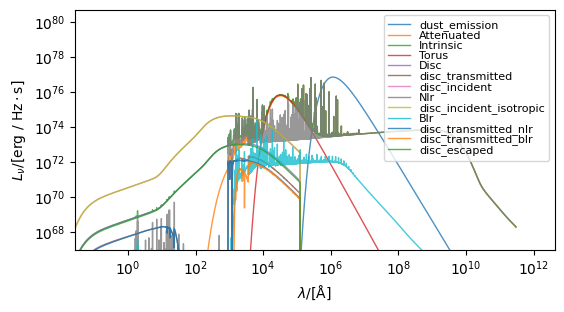
Integrating spectra

The integrated spectra are automatically produced alongside per particle spectra. However, if we wanted to explictly get the integrated spectra from the particle spectra we just generated (for instance if we had made some modification after generation), we can call the integrate_particle_spectra method. This method will sum the individual spectra and populate the spectra dictionary.

Note, we can also integrate individual spectra using the Sed.sum() method.

print(blackholes.spectra)
blackholes.integrate_particle_spectra()
print(blackholes.spectra)

fig, ax = blackholes.plot_spectra(show=True, figsize=(6, 4))

{'disc_transmitted_blr': <synthesizer.sed.Sed object at 0x7f032b9f4430>, 'disc_transmitted_nlr': <synthesizer.sed.Sed object at 0x7f0337984820>, 'disc_escaped': <synthesizer.sed.Sed object at 0x7f03199768f0>, 'blr': <synthesizer.sed.Sed object at 0x7f03199770a0>, 'nlr': <synthesizer.sed.Sed object at 0x7f0319977370>, 'disc_incident_isotropic': <synthesizer.sed.Sed object at 0x7f0319976ec0>, 'disc_incident': <synthesizer.sed.Sed object at 0x7f0319977100>, 'disc_transmitted': <synthesizer.sed.Sed object at 0x7f03199771f0>, 'disc': <synthesizer.sed.Sed object at 0x7f0319974cd0>, 'torus': <synthesizer.sed.Sed object at 0x7f0319976a40>, 'intrinsic': <synthesizer.sed.Sed object at 0x7f0319976ef0>, 'attenuated': <synthesizer.sed.Sed object at 0x7f0319976dd0>, 'dust_emission': <synthesizer.sed.Sed object at 0x7f0319976350>}
{'disc_transmitted_blr': <synthesizer.sed.Sed object at 0x7f033790c970>, 'disc_transmitted_nlr': <synthesizer.sed.Sed object at 0x7f032b9f4430>, 'disc_escaped': <synthesizer.sed.Sed object at 0x7f0337984820>, 'blr': <synthesizer.sed.Sed object at 0x7f031f92df30>, 'nlr': <synthesizer.sed.Sed object at 0x7f031994d570>, 'disc_incident_isotropic': <synthesizer.sed.Sed object at 0x7f031f92e2c0>, 'disc_incident': <synthesizer.sed.Sed object at 0x7f031f92db70>, 'disc_transmitted': <synthesizer.sed.Sed object at 0x7f031f92e980>, 'disc': <synthesizer.sed.Sed object at 0x7f031f92da20>, 'torus': <synthesizer.sed.Sed object at 0x7f031f92e440>, 'intrinsic': <synthesizer.sed.Sed object at 0x7f031f92e3e0>, 'attenuated': <synthesizer.sed.Sed object at 0x7f031f92ddb0>, 'dust_emission': <synthesizer.sed.Sed object at 0x7f031f92de10>}

Modifying EmissionModel parameters with get_spectra

As well as modifying a model explicitly, it’s also possible to overide the properties of a model at the point get_spectra is called. These modifications will not be remembered by the model afterwards. As it stands, this form of modification is supported for the dust_curve, tau_v, covering_fraction and masks.

Here we’ll demonstrate this by overiding the covering fractions to generate spectra for a range of covering_fraction values. This can either be done by passing a single number which will overide all covering fractions on every model (probably undesirable behaviour since this will set NLR and BLR covering fractions to be equal).

# Since we now want integrated spectra lets remove the per particle flag
dust_model.set_per_particle(False)

blackhole.clear_all_spectra()
spectra = {}
for fesc in [0.1, 0.5, 0.9]:
    blackhole.get_spectra(dust_model, covering_fraction=fesc)
    spectra[r"$f " f"=$ {fesc}"] = blackhole.spectra["intrinsic"]

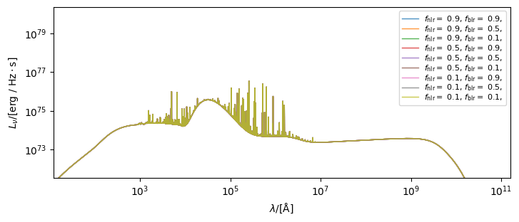
Or (more desirably) we can pass a dictionary mapping model labels to fesc values to target specific models. Notice that we have invoked the clear_all_spectra method to reset the spectra dictionary, we can also clear all emissions (including spectra, lines, and photometry if they are present) with the clear_all_emissions method.

blackhole.clear_all_emissions()
spectra = {}
for nlr_fesc in [0.1, 0.5, 0.9]:
    for blr_fesc in [0.1, 0.5, 0.9]:
        blackhole.get_spectra(
            dust_model,
            covering_fraction={
                "disc_transmitted_nlr": nlr_fesc,
                "disc_transmitted_blr": blr_fesc,
            },
        )
        spectra[
            r"$f_\mathrm{nlr} "
            f"=$ {nlr_fesc}, "
            r"$f_\mathrm{blr} "
            f"=$ {blr_fesc},"
        ] = blackhole.spectra["intrinsic"]

To see the variation above we can pass the dictionary we populated with the varied spectra to the plot_spectra function (where the dictionary keys will be used as labels).

from synthesizer.sed import plot_spectra

plot_spectra(spectra, figsize=(8, 4))

(<Figure size 800x400 with 1 Axes>,
 <Axes: xlabel='$\\lambda/[\\mathrm{\\AA}]$', ylabel='$L_{\\nu}/[\\mathrm{\\rm{erg} \\ / \\ \\rm{Hz \\cdot \\rm{s}}}]$'>)