Images From Galaxy Particle distributions

Synthesizer can create various different types of images and maps from particle data.

In the example below we demonstrate this for a galaxy stellar distribution taken from a CAMELS simulation galaxy.

import time

import matplotlib.colors as cm
import matplotlib.gridspec as gridspec
import matplotlib.pyplot as plt
import numpy as np
from astropy.cosmology import Planck18 as cosmo
from scipy import signal
from unyt import Hz, angstrom, erg, kpc, s

from synthesizer.emission_models import BimodalPacmanEmission
from synthesizer.emission_models.attenuation import PowerLaw
from synthesizer.filters import FilterCollection as Filters
from synthesizer.grid import Grid
from synthesizer.kernel_functions import Kernel
from synthesizer.load_data.load_camels import load_CAMELS_IllustrisTNG

# Define the grid
grid_name = "test_grid"
grid_dir = "../../../tests/test_grid/"
grid = Grid(
    grid_name, grid_dir=grid_dir, new_lam=np.logspace(2, 5, 600) * angstrom
)

# Create galaxy object
gal = load_CAMELS_IllustrisTNG(
    "../../../tests/data/",
    snap_name="camels_snap.hdf5",
    group_name="camels_subhalo.hdf5",
    physical=True,
)[1]

Getting the photometry

To make an image we need to generate spectra for each individual star particle. To do this we use the galaxy’s in built get_spectra method and pass a per_particle model. This will generate a spectrum for each particle in the galaxy.

We can then calculate the photometry on these spectra by defining a filter collection, and calculating the luminosities.

# Get the stellar pacman model
model = BimodalPacmanEmission(
    grid=grid,
    tau_v_ism=1.0,
    tau_v_birth=0.7,
    dust_curve_ism=PowerLaw(slope=-1.3),
    dust_curve_birth=PowerLaw(slope=-0.7),
    # dust_emission_ism=Blackbody(temperature=100 * kelvin),
    # dust_emission_birth=Blackbody(temperature=30 * kelvin),
    fesc=0.1,
    fesc_ly_alpha=0.9,
    label="total",
    per_particle=True,
)

# And use it to generate the spectra
sed = gal.stars.get_spectra(model)

# Get the observed spectra
gal.get_observed_spectra(cosmo)

# Set up the filter collection for imaging
filter_codes = [
    "JWST/NIRCam.F090W",
    "JWST/NIRCam.F150W",
    "JWST/NIRCam.F200W",
]
filters = Filters(filter_codes, new_lam=grid.lam)

gal.get_photo_lnu(filters)

Imaging

The last step before we can make any images is to define the resolution of our images and the FOV (or width) of the images. These must have units associated to them to enable the code to internally transform all quantites to a consistent unit system.

# Define the width of the image
width = 30 * kpc

# Define image resolution (here we arbitrarily set it to 100
# pixels along an axis)
resolution = width / 200

print(
    "Image width is %.2f kpc with %.2f kpc resolution"
    % (width.value, resolution.value)
)

Image width is 30.00 kpc with 0.15 kpc resolution

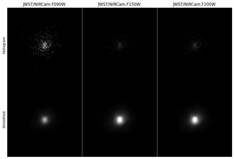
Now we have everything we need to make images. Although it is possible to work with the low level ImageCollection and Image methods, here we use the interface on a Galaxy. There are two of these helper methods, get_imgs_luminosity for luminosity images, and get_imgs_flux for flux images. We will focus on the former here.

The image helper methods both take the image properties we previously defined, and a spectra type. These types can be any spectra for which you have calculated photometry, e.g. "incident", "intrinsic", or "attenuated", for either stars (stellar_photometry) or black holes (blackhole_photometry). If both a stellar and black hole photometry type are passed then an image is made for each component before they are combined and returned.

Images can either be simple 2D histograms, or the particles can be smoothed over their kernels. What type of image is made is controlled by the img_type argument. Below we demonstrate both approaches. However, for the latter we also need to define a kernel, which we have already imported from the kernel_functions module.

# Get the SPH kernel
sph_kernel = Kernel()
kernel_data = sph_kernel.get_kernel()

# Get the image
hist_imgs = gal.get_images_luminosity(
    resolution=resolution,
    fov=width,
    emission_model=model,
    img_type="hist",
    limit_to="nebular",  # we can limit to a single image type
)

# Get the image
smooth_imgs = gal.get_images_luminosity(
    resolution,
    fov=width,
    emission_model=model,
    img_type="smoothed",
    kernel=kernel_data,
    kernel_threshold=1,
)

When making images in multiple bands, the image arrays themselves are stored on the returned ImageCollection in a dictionary called imgs, of the form {filter_code: Image}. Here, an Image is a container including the image array itself (arr), unit information (units) and the resolution and fov of the image. An Image object also includes a number of different methods for manipulating and visualising individual images.

Below we will extract this dictionary and plot each of the images we have made.

# Lets set up a simple normalisation across all images
vmax = 0
for img in hist_imgs.values():
    up = np.percentile(img.arr, 99.9)
    if up > vmax:
        vmax = up
hist_norm = cm.Normalize(vmin=0, vmax=vmax)
vmax = 0
for img in smooth_imgs.values():
    up = np.percentile(img.arr, 99.9)
    if up > vmax:
        vmax = up
smooth_norm = cm.Normalize(vmin=0, vmax=vmax)


# Set up plot
fig = plt.figure(figsize=(4 * len(filters), 4 * 2))
gs = gridspec.GridSpec(2, len(filters), hspace=0.0, wspace=0.0)

# Create top row
axes = []
for i in range(len(filters)):
    axes.append(fig.add_subplot(gs[0, i]))

# Loop over images plotting them
for ax, fcode in zip(axes, filter_codes):
    ax.imshow(hist_imgs[fcode].arr, norm=hist_norm, cmap="Greys_r")
    ax.set_title(fcode)
    ax.tick_params(
        axis="both",
        which="both",
        left=False,
        right=False,
        labelleft=False,
        labelright=False,
        bottom=False,
        top=False,
        labelbottom=False,
        labeltop=False,
    )

# Set y axis label on left most plot
axes[0].set_ylabel("Histogram")

# Create bottom row
axes = []
for i in range(len(filters)):
    axes.append(fig.add_subplot(gs[1, i]))

# Loop over images plotting them
for ax, fcode in zip(axes, filter_codes):
    ax.imshow(smooth_imgs[fcode].arr, norm=smooth_norm, cmap="Greys_r")
    ax.tick_params(
        axis="both",
        which="both",
        left=False,
        right=False,
        labelleft=False,
        labelright=False,
        bottom=False,
        top=False,
        labelbottom=False,
        labeltop=False,
    )

# Set y axis label on left most plot
axes[0].set_ylabel("Smoothed")

# Plot the image
plt.show()
plt.close(fig)

Applying a Point Spread Function (PSF)

To properly model observations from a particular instrument we must take into account the point spread function (PSF).

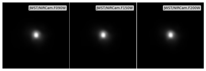
To apply a PSF we can either use Image.apply_psf on individual Image objects, or apply a dictionary of PSFs, of the form {filter_code: psf_array}, to each image in an ImageCollection with the apply_psfs method. Here we will just create a fake gaussian PSF for all filters, but PSFs can be sourced however the user wishes (for Webb we recommend the webbpsf package), as long as a simple numpy array is passed within the psf dictionary for each filter.

To get the most accurate result from the PSF convolution it is recommended to do the convolution on a super-sampled image (i.e. much higher resolution than the PSF). Although-here we just supersample the images we have already made, it is recommended to first make the images at the super-sampled resolution, and then subsequently downsample after the fact.

# Create a fake PSF for each filter
psf = np.outer(
    signal.windows.gaussian(100, 3), signal.windows.gaussian(100, 3)
)
psfs = {f: psf for f in filters.filter_codes}

# Supersample the image
smooth_imgs.supersample(2)

# Apply the PSFs
psf_imgs = smooth_imgs.apply_psfs(psfs)

# And downsample back to the native resolution
smooth_imgs.downsample(0.5)
psf_imgs.downsample(0.5)

apply_psfs returns a new ImageCollection containing the newly convolved Image objects. We can now use the plotting helper function to plot these images, with some normalisation.

# Lets set up a simple normalisation across all images
vmax = 0
for img in psf_imgs.values():
    up = np.percentile(img.arr, 99.9)
    if up > vmax:
        vmax = up

# Get the plot
fig, ax = psf_imgs.plot_images(show=True, vmin=0, vmax=vmax)
plt.close(fig)

Applying noise

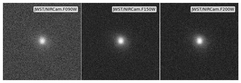
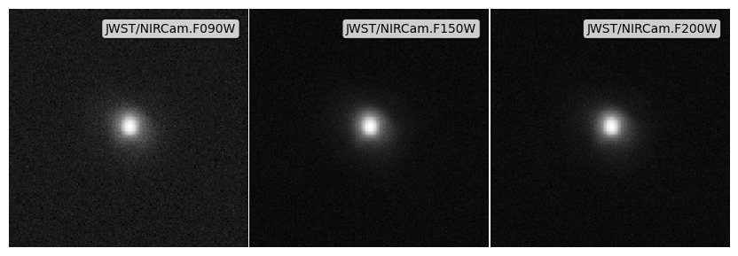
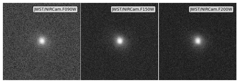
The final ingredient for a fully forward modelled synthetic image is a noise field. We include 4 different to approaches to include noise: - apply_noise_array: Add an existing noise field / array. - apply_noise_from_std: Derive a noise distribution, centered on 0, given a user specified standard deviation, and then generate and add a noise array. - apply_noise_from_snr (aperture): Derive a noise distribution from a Signal-to-Noise Ratio (SNR), defined in an aperture with size aperture_radius and a specified depth. This will derive the standard deviation of the noise distribution assuming \(SNR= S / \sigma\) for an aperture, before deriving the per pixel noise, computing the noise array and adding it. - apply_noise_from_snr (point source): Derive a noise distribution from a SNR and depth. This will derive the standard deviation of the noise distribution assuming \(SNR= S / \sigma\) for a pixel before computing the noise array and adding it. This behaviour can be achieved by omitting aperture_radius in the call to apply_noise_from_snr

As with applying a PSF, these methods have singular versions (as listed above) which can be used on an individual Image, and pluralised versions which can be used on an ImageCollection, and take dictionaries for each of the arguments.

If an image has units then the passed noise_arr or noise_std must also have units.

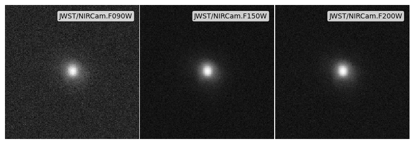
Applying noise with any of the methods described above will return a new ImageCollection / Image containing the noisy image. In addition to the noisy image (stored under Image.arr) the new Image (or the new Image objects within an ImageCollection) will contain the noise array stored in the noise_arr attribute, and the weight map stored in the weight_map attribute on the Image.

Below we demonstrate each method using the ImageCollection interface. The noise and weight maps are stored in Image.noise_arr and Image.weight_map.

Noise arrays

img_start = time.time()

# Get a noise array for each filter
noises = {
    f: np.random.normal(loc=0, scale=10**26.0, size=(psf_imgs.npix))
    * erg
    / s
    / Hz
    for f in psf_imgs.keys()
}

# Apply the noise array
noise_array_imgs = psf_imgs.apply_noise_arrays(noises)

print("Noisy images made, took:", time.time() - img_start)

# Get the plot
fig, ax = noise_array_imgs.plot_images(show=True, vmin=0, vmax=vmax)
plt.close(fig)

Noisy images made, took: 0.01079106330871582

Noise from standard deviations

img_start = time.time()

# Get a noise standard deviation for each filter
noise_stds = {f: 10**26.3 * erg / s / Hz for f in psf_imgs.keys()}

# Apply the noise array
noise_std_imgs = psf_imgs.apply_noise_from_stds(noise_stds)

print("Noisy images made, took:", time.time() - img_start)

# Get the plot
fig, ax = noise_std_imgs.plot_images(show=True, vmin=0, vmax=vmax)
plt.close(fig)

Noisy images made, took: 0.0048067569732666016

Noise from an aperture depth

# Get dictionaries with the noise properties for each filter
snrs = {f: 5 for f in psf_imgs.keys()}
depths = {f: 10**28.0 * erg / s / Hz for f in psf_imgs.keys()}

# Apply the noise array
noise_app_imgs = psf_imgs.apply_noise_from_snrs(
    snrs=snrs, depths=depths, aperture_radius=0.5 * kpc
)

print("Noisy images made, took:", time.time() - img_start)

# Get the plot
fig, ax = noise_app_imgs.plot_images(show=True, vmin=0, vmax=vmax)
plt.close(fig)

Noisy images made, took: 0.1344747543334961

Noise from point source depth

# Get dictionaries with the noise properties for each filter
snrs = {f: 5 for f in psf_imgs.keys()}
depths = {f: 10**27.0 * erg / s / Hz for f in psf_imgs.keys()}

# Apply the noise array
noise_ps_imgs = psf_imgs.apply_noise_from_snrs(snrs=snrs, depths=depths)

print("Noisy images made, took:", time.time() - img_start)

# Get the plot
fig, ax = noise_ps_imgs.plot_images(show=True, vmin=0, vmax=vmax)
plt.close(fig)

Noisy images made, took: 0.25371789932250977

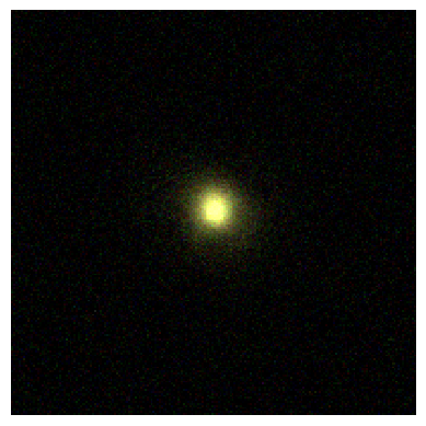
Making an RGB image

Finally we can use the RGB image method on the ImageCollection to make quick RGB images by simply providing a dictionary detailing which filters we want in which bands, and optional weights for each filter (which we will ignore here).

# Create the rgb image from the psf image above example using our 3 filters
rgb_img = noise_ps_imgs.make_rgb_image(
    rgb_filters={
        "R": [
            "JWST/NIRCam.F200W",
        ],
        "G": [
            "JWST/NIRCam.F150W",
        ],
        "B": [
            "JWST/NIRCam.F090W",
        ],
    },
)

# Set up minima and maxima
vmin = -np.percentile(rgb_img, 32)
vmax = np.percentile(rgb_img, 99.9)
norm = cm.Normalize(vmin=vmin, vmax=vmax, clip=True)
print("Scaling to:", vmin, "->", vmax)

# Normalise the image.
rgb_img = norm(rgb_img)

print(rgb_img.shape)

# Plot the image
fig = plt.figure()
ax = fig.add_subplot(111)
ax.imshow(rgb_img, origin="lower", interpolation="nearest")
ax.axis("off")
plt.show()
plt.close(fig)

Scaling to: 4.817079333790617e+25 -> 9.045685773970884e+27
(200, 200, 3)

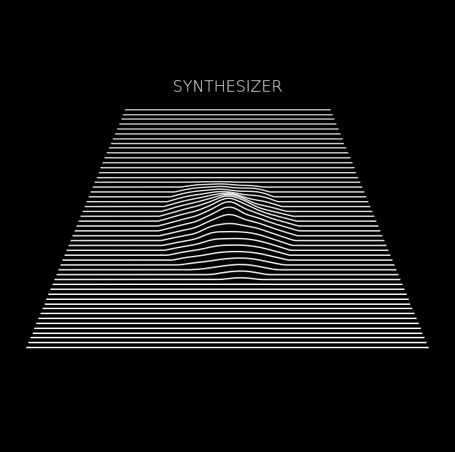
Unknown Pleasures

This functionality needs very little explanation. If you like Joy Division you already know.

psf_imgs["JWST/NIRCam.F200W"].plot_unknown_pleasures()

(<Figure size 800x800 with 1 Axes>, <Axes: >)