Dust emission

Synthesizer can model thermal dust emission using an energy balance approach. This is done using dust emission models, which can then be handed to an EmissionModel to produce a dust emission spectrum, which can be combined with any other spectra in the model.

First we load some common modules, and define a wavelength array over which we will generate our dust emission SED

import matplotlib.pyplot as plt
import numpy as np
from unyt import Angstrom, K, Lsun, Msun, um

from synthesizer.emission_models.dust.emission import (
    Blackbody,
    Casey12,
    Greybody,
    IR_templates,
)

lam = 10 ** (np.arange(3.0, 8.0, 0.01)) * Angstrom

Parametric models

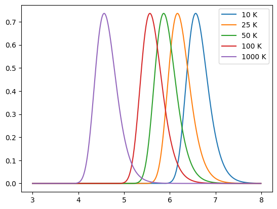
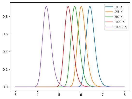
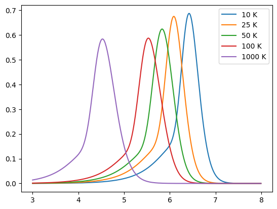
Below we show a number of simple models, including a blackbody, greybody (non-unity emissivity) and the model detailed in Casey et al. (2012). By default a dust emission model provides a normalised spectrum.

for T in [10, 25, 50, 100, 1000]:
    model = Blackbody(T * K)
    sed = model.get_spectra(lam)
    plt.plot(np.log10(sed.lam), sed.luminosity, label=f"{T} K")

plt.legend()
plt.show()

for T in [10, 25, 50, 100, 1000]:
    model = Greybody(T * K, 1.6)
    sed = model.get_spectra(lam)
    plt.plot(np.log10(sed.lam), sed.luminosity, label=f"{T} K")

plt.legend()
plt.show()

for T in [10, 25, 50, 100, 1000]:
    model = Casey12(T * K, 1.6, 2.0)
    sed = model.get_spectra(lam)
    plt.plot(np.log10(sed.lam), sed.luminosity, label=f"{T} K")

plt.legend()
plt.show()

[8, 1000] * um

unyt_array([   8, 1000], 'μm')

Adding CMB heating

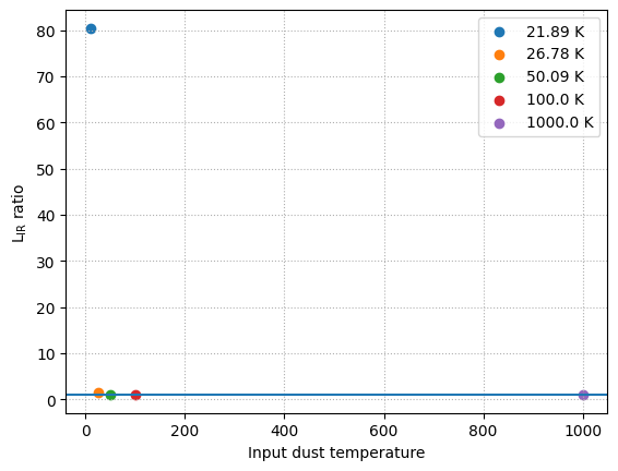
At high redshift, the effect of CMB heating is important. To account for this any dust emission model can incorporate the impact of CMB heating (cmb_heating) at a given redshift (\(z\)). Below we compare the dust emission spectrum from the Casey+12 model with and without CMB heating:

for T in [10, 25, 50, 100, 1000]:
    model = Casey12(T * K, 1.6, 2.0)
    model_cmb = Casey12(T * K, 1.6, 2.0, cmb_heating=True, redshift=7)
    sed = model.get_spectra(lam)
    sed_cmb = model_cmb.get_spectra(lam)
    L_ir_ratio = sed_cmb.measure_window_luminosity(
        window=[8, 1000] * um
    ) / sed.measure_window_luminosity(
        window=[8, 1000] * um
    )  # same as model_cmb.cmb_factor
    plt.scatter(
        T, L_ir_ratio, label=f"{np.around(model_cmb.temperature_z, 2)}"
    )

plt.axhline(y=1)
plt.grid(ls="dotted")
plt.xlabel("Input dust temperature")
plt.ylabel(r"L$_{\rm IR}$ ratio")
plt.legend()
plt.show()

IR Templates

Draine & Li 2007 dust models

The more complex model present in Draine & Li 2007 is also available; this requires a grid to be loaded in.

Begin by reading in the DL07 grids, which have been created by downloading the ASCII DL07 files and running

from synthesizer.utils import process_dl07_to_hdf5
process_dl07_to_hdf5()

However, you can download these preprocessed grids using the synthesizer-download command line tool.

synthesizer-download -d /path/to/destination --dust-grid

from synthesizer.grid import Grid

grid_name = "MW3.1"
grid_dir = "../../../tests/test_grid/"
grid = Grid(grid_name, grid_dir=grid_dir, read_lines=False)
print(grid.axes)

['qpah', 'umin', 'alpha']

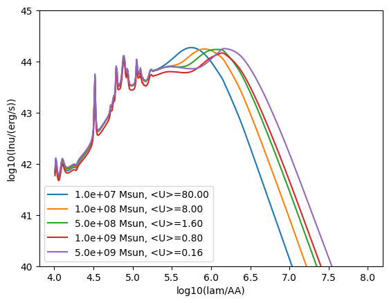
Below we show how to use the DL07 model directly, and plot the dust emission spectrum for a number of dust luminosities. You can also pass these models to an EmissionModel and they will be used automatically.

for mdust in [1e7, 1e8, 5e8, 1e9, 5e9]:
    model = IR_templates(
        grid, mdust=mdust * Msun, ldust=1e11 * Lsun, verbose=False
    )
    sed = model.get_spectra(lam)
    plt.plot(
        np.log10(sed.lam),
        np.log10(sed.luminosity),
        label="{:.1e} Msun, <U>={:.2f}".format(mdust, model.u_avg),
    )

plt.xlabel("log10(lam/AA)")
plt.ylabel("log10(lnu/(erg/s))")
plt.ylim(40, 45)
plt.legend()
plt.show()