Camels example

Use test cosmological simulation data (from the [CAMELS simulations]( https://www.camel-simulations.org/)) to generate spectra and calculate photometry.

• 
• 
• 
• 
• 
• 
• 
• 
• 
• 

Loaded 10 galaxies
--------------------------------------------------
|               PHOTOMETRY (FLUX)                |
|--------------------|---------------------------|
| U (λ = 3.65e+03 Å) | 2.89e-13 erg/(Hz*cm**2*s) |
|--------------------|---------------------------|
| V (λ = 5.50e+03 Å) | 1.79e-12 erg/(Hz*cm**2*s) |
|--------------------|---------------------------|
| J (λ = 1.22e+04 Å) | 4.76e-12 erg/(Hz*cm**2*s) |
--------------------------------------------------

--------------------------------------------------
|               PHOTOMETRY (FLUX)                |
|--------------------|---------------------------|
| U (λ = 3.65e+03 Å) | 1.87e-13 erg/(Hz*cm**2*s) |
|--------------------|---------------------------|
| V (λ = 5.50e+03 Å) | 1.28e-12 erg/(Hz*cm**2*s) |
|--------------------|---------------------------|
| J (λ = 1.22e+04 Å) | 3.94e-12 erg/(Hz*cm**2*s) |
--------------------------------------------------

Stellar luminosities available: ['incident', 'old_incident', 'young_incident', 'nebular', 'nebular_continuum', 'nebular_line', 'transmitted', 'reprocessed', 'attenuated', 'young_transmitted', 'young_nebular', 'old_nebular', 'old_transmitted', 'young_intrinsic', 'young_emergent', 'old_intrinsic', 'old_emergent', 'young_reprocessed', 'young_attenuated_nebular', 'young_attenuated', 'old_reprocessed', 'old_attenuated', 'intrinsic', 'young_attenuated_ism', 'emergent']
Stellar fluxes available: ['incident', 'old_incident', 'young_incident', 'nebular', 'nebular_continuum', 'nebular_line', 'transmitted', 'reprocessed', 'attenuated', 'young_transmitted', 'young_nebular', 'old_nebular', 'old_transmitted', 'young_intrinsic', 'young_emergent', 'old_intrinsic', 'old_emergent', 'young_reprocessed', 'young_attenuated_nebular', 'young_attenuated', 'old_reprocessed', 'old_attenuated', 'intrinsic', 'young_attenuated_ism', 'emergent']

import matplotlib.pyplot as plt
import numpy as np
from astropy.cosmology import Planck18 as cosmo
from unyt import Myr, dimensionless

from synthesizer.emission_models import (
    AttenuatedEmission,
    CharlotFall2000,
    IncidentEmission,
    NebularEmission,
    ReprocessedEmission,
    StellarEmissionModel,
)
from synthesizer.emission_models.attenuation import PowerLaw
from synthesizer.filters import UVJ
from synthesizer.grid import Grid
from synthesizer.load_data.load_camels import load_CAMELS_IllustrisTNG
from synthesizer.sed import Sed, plot_spectra

# Get the grid
grid_dir = "../../tests/test_grid"
grid_name = "test_grid"
grid = Grid(grid_name, grid_dir=grid_dir)


# We then need to load our galaxy data. There are custom data loading
# script for different simulation codes in `synthesizer.load_data`. For
# CAMELS-IllutrisTNG there is the `load_CAMELS_IllutrisTNG` method
#
# If your simulation does not have its own front end, please use the
# templates in `synthesizer/load_data.py` to create your own.
gals = load_CAMELS_IllustrisTNG(
    "../../tests/data/",
    snap_name="camels_snap.hdf5",
    group_name="camels_subhalo.hdf5",
)

print(f"Loaded {len(gals)} galaxies")

# this creates `gals`, which is a list containing a `synthesizer.Galaxy`
# object for each structure in the subfind file. These `Galaxy` objects
# contain lots of useful methods for acting on galaxies, in addition to
# the component parts of a galaxy. These components include `Stars`, `Gas
# `, and `BlackHoles`.

# Lets take a galaxy to work with
g = gals[1]

# Before we can generate any spectra we need to instantiate an emission model.
# To begin with lets just use a premade incident model to get the
# incident stellar spectra.
incident = IncidentEmission(grid)

# To get a spectra we just call the `get_spectra` method on the stars with
# whatever emission model we want to use, here the incident model.
spec = g.stars.get_spectra(incident)

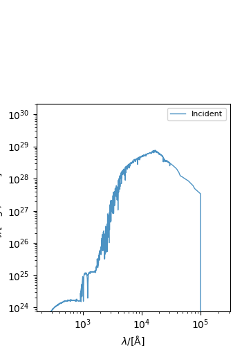
# Lets use the `stars.plot_spectra` method to plot this spectra. This method
# can either plot all spectra on a component or a specific subset if desired.
g.stars.plot_spectra(show=True)

# Why might you want to create an `Sed` object? This class contains a lot
# of useful functionality for working with SED's. For example, we can
# calculate the broadband luminosities.
#
# First, get rest frame 'flux' from the `Sed`.
spec.get_fnu0()

# To get broadband luminosity we first need to define a filter collection
# object (UVJ default).
fc = UVJ(new_lam=grid.lam)

# And then we can apply it using the `Sed` helper function.
_UVJ = spec.get_photo_fnu(fc)
print(_UVJ)

# ## Young and old stellar populations
#
# We can also restrict the age of star particles used for calculating the
# spectra. To do this we simply supply the emission model with a mask. Lets
# use incident emission as another example.
young_incident = IncidentEmission(
    grid,
    label="young_incident",
    mask_attr="ages",
    mask_thresh=100 * Myr,
    mask_op="<",
)
old_incident = IncidentEmission(
    grid,
    label="old_incident",
    mask_attr="ages",
    mask_thresh=100 * Myr,
    mask_op=">=",
)

# If we also want the total incident emission we can also combine the young
# and old emission and then feed this model to the spectra method to get
# all 3 spectra at once.
combined_incident = StellarEmissionModel(
    grid=grid,
    label="incident",
    combine=(young_incident, old_incident),
)
combined_spec = g.stars.get_spectra(combined_incident)

# Once again we can plot them all
g.stars.plot_spectra(show=True)

# ### Replacing young star particles with Parametric Star Formation Histories
#
# For simulations with low mass resolution, the sampling of the star
# formation history can be affected by Poisson scatter. This is
# particularly the case for young star particles; a single massive
# particle that happens to form close to the time of observation can
# significantly alter the integrated colour of the entire galaxy.
#
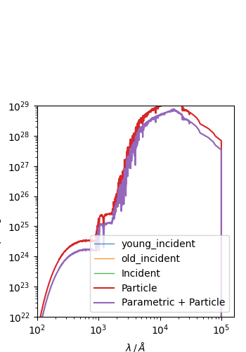
# To mitigate this, we provide a method for smoothing the recent star
# formation history of a particle galaxy by replacing each young star
# particle with a parametric SFH.
#
# This by calling parametric_young_stars on the Stars object. This method
# will replace the young star particles with particles sampled from a
# parametric SFH. The method requires the age below which to replace the
# particles, the parametric SFH to use, and the grid to use for the
# parametric SFH.
g.stars.parametric_young_stars(
    age=500 * Myr,
    parametric_sfh="constant",
    grid=grid,
)
parametric_spec = g.stars.get_spectra(incident)
plot_spectra(
    {"Particle": spec, "Parametric + Particle": parametric_spec},
    show=True,
)


# ## Nebular emission
#
# If our grid file has been post-processed with CLOUDY we can produce the
# nebular emission for our camels galaxies. For this we need get a
# NebularEmissionModel
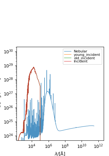
nebular = NebularEmission(grid)

# And then, like before, we just hand this off to the `plot_spectra` method
spec = g.stars.get_spectra(nebular)
fig, ax = g.stars.plot_spectra(show=True)

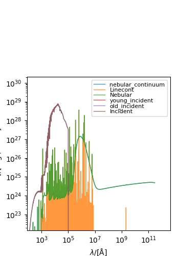
# With any of the spectra we've made so far we could also pass an escape
# fraction (fesc) but specifically for nebular we will get extra line and
# nebular emission if we pass a lyman alpha escape fraction.
nebular = NebularEmission(grid, fesc_ly_alpha=0.2)
spec = g.stars.get_spectra(nebular)
fig, ax = g.stars.plot_spectra(show=True)

# To get the gas reprocessed spectra, which
# we refer to as the *reprocessed* spectra, assuming some escape fraction
# `fesc`.
reprocessed = ReprocessedEmission(
    grid,
    fesc=0.2,
    fesc_ly_alpha=0.1,
)
g.stars.get_spectra(reprocessed)

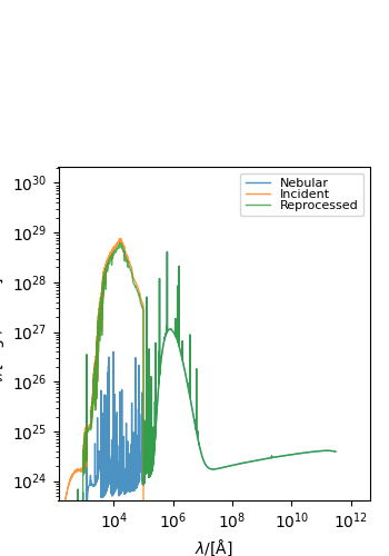
# The plots starting to get a bit messy now so let's select the spectra we
# want to plot
fig, ax = g.stars.plot_spectra(
    show=True,
    spectra_to_plot=("reprocessed", "incident", "nebular"),
)

# ## Dust attenuation
#
# We can apply a range of different dust models to our reprocessed spectra. To
# do so we can simply make an attenuated model and point it at our reprocessed
# model. To do so we need a dust_curve, for more details on these see the
# dust attenuation docs.
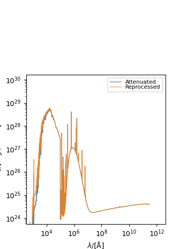
attenuated = AttenuatedEmission(
    grid=grid,
    emitter="stellar",
    dust_curve=PowerLaw(slope=-1),
    apply_dust_to=reprocessed,
    tau_v=0.33,
    component="stellar",  # we can point models at different components
)
spec = g.stars.get_spectra(attenuated)
fig, ax = g.stars.plot_spectra(
    show=True,
    spectra_to_plot=["reprocessed", "attenuated"],
)

# Of course, in reality we won't be making individual models and calling
# get_spectra with them 1 by 1. Instead we can make/use large models
# which will generate all the spectra we want at once. For more details
# on making your own models see the emisison models docs. Here we will
# use a premade model that will produce spectra following Charlot&Fall2000
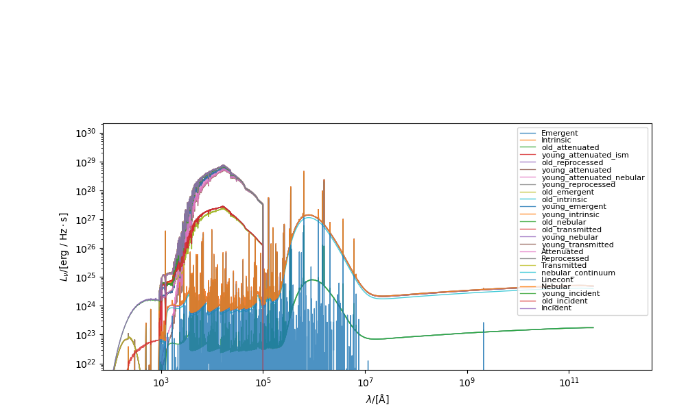
cf_model = CharlotFall2000(
    grid,
    tau_v_ism=0.33,
    tau_v_birth=0.67,
    dust_curve_ism=PowerLaw(slope=-0.7),
    dust_curve_birth=PowerLaw(slope=-1.3),
    age_pivot=10 * dimensionless,
)
spec = g.stars.get_spectra(cf_model)
fig, ax = g.stars.plot_spectra(show=True, figsize=(10, 6))


# ### Multiple galaxies
# If we want to create spectra for multiple galaxies and then interact with
# a particular spectra from them all in a single Sed object we can use a list
# comprehension. Here we grab the luminosity `lnu` of each galaxy into a
# list, and combine into a single sed object afterwards using the grid
# wavelength.
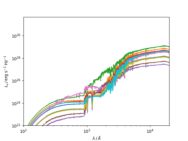
specs = np.vstack([g.stars.get_spectra(incident).lnu for g in gals])
specs = Sed(lam=grid.lam, lnu=specs)


# Importantly here, we don't create an SED object for each galaxy spectra
# . We instead create the 2D array of spectra, and then create an `Sed`
# object for the whole collection.
fig, ax = plt.subplots(1, 1)
ax.loglog(grid.lam, specs.lnu.T)
ax.set_ylim(
    1e22,
)
ax.set_xlim(1e2, 2e4)
ax.set_xlabel("$\\lambda \\,/\\, \\AA$")
ax.set_ylabel("$L_{\\nu} \\,/\\, \\mathrm{erg \\; s^{-1} \\; Hz^{-1}}$")


# ### Calculate broadband luminosities
#
# We can then use the `Sed` methods on the whole collection. This is much
# faster than calling the method for each spectra individually, since we
# can take advantage of vectorisation. For example, we can calculate UVJ
# colours of all the selected galaxies in just a couple of lines.
#
# First get rest frame 'flux'


spec.get_fnu0()


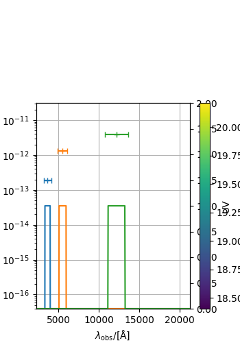
# Define a filter collection object (UVJ default) and calculate the photometry.


fc = UVJ(new_lam=grid.lam)

_UVJ = spec.get_photo_fnu(fc)
print(_UVJ)
_UVJ.plot_photometry(show=True)


# Do for multiple, plot UVJ diagram, coloured by $M_{\star}$


mstar = np.log10(
    np.array([np.sum(g.stars.initial_masses) for g in gals]) * 1e10
)


specs.get_fnu0()
_UVJ = specs.get_photo_fnu(fc)

UV = _UVJ["U"] / _UVJ["V"]
VJ = _UVJ["V"] / _UVJ["J"]

plt.scatter(VJ, UV, c=mstar, s=40)
plt.xlabel("VJ")
plt.ylabel("UV")
plt.colorbar(
    label=r"$\mathrm{log_{10}} \, M_{\star} \,/\, \mathrm{M_{\odot}}$"
)


# ## Collective operations
#
# It is often useful to collectively do different operations on a `Galaxy
# `. Synthesizer enables this via some wrapper methods on a galaxy which
# will operate on it's components to, for instance, get the observed
# spectra or photometry for all spectra nested in a `Galaxy`.

# Get observed spectra for all spectra
g.get_observed_spectra(cosmo=cosmo)

# Get UVJ photometry for all spectra
g.get_photo_lnu(fc)
g.get_photo_fnu(fc)

print("Stellar luminosities available:", list(g.stars.photo_lnu.keys()))
print("Stellar fluxes available:", list(g.stars.photo_fnu.keys()))