Compare SPS grid assignment methods

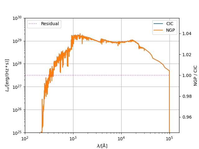
This example compares a the cloud in cell (CIC) and nearest grid point (NGP) grid assignment methods. These methods dictate how mass is assigned to spectra in the SPS grids.

import matplotlib.pyplot as plt
from unyt import Msun, Myr

from synthesizer.emission_models import IncidentEmission
from synthesizer.grid import Grid
from synthesizer.parametric import SFH, ZDist
from synthesizer.parametric import Stars as ParametricStars
from synthesizer.particle.galaxy import Galaxy as ParticleGalaxy
from synthesizer.particle.stars import sample_sfzh

# Define the grid
grid_name = "test_grid"
grid_dir = "../../tests/test_grid/"
grid = Grid(grid_name, grid_dir=grid_dir)

# Define the emission model
model = IncidentEmission(grid)

# Define the SFH and metallicity distribution
Z_p = {"metallicity": 0.01}
metal_dist = ZDist.DeltaConstant(**Z_p)
sfh_p = {"duration": 100 * Myr}
sfh = SFH.Constant(**sfh_p)

# Define the parametric stars
sfzh = ParametricStars(
    grid.log10age,
    grid.metallicity,
    sf_hist=sfh,
    metal_dist=metal_dist,
    initial_mass=10**9 * Msun,
)

# How many particles?
nstar = 10**5

# Get the stars object
stars = sample_sfzh(
    sfzh.sfzh,
    sfzh.log10ages,
    sfzh.log10metallicities,
    nstar,
    initial_mass=10**9 / nstar * Msun,
)

# Create galaxy object
particle_galaxy = ParticleGalaxy(stars=stars)

# Calculate the stars SEDs using both grid assignment schemes
cic_sed = particle_galaxy.stars.get_spectra(
    model,
    grid_assignment_method="cic",
)
ngp_sed = particle_galaxy.stars.get_spectra(
    model,
    grid_assignment_method="ngp",
)

# Setup the plot
fig = plt.figure()
ax = fig.add_subplot(111)
resi_ax = ax.twinx()
ax.grid(True)

resi_ax.semilogx(
    ngp_sed.lam,
    ngp_sed.lnu / cic_sed.lnu,
    color="m",
    linestyle="dotted",
    label="Residual",
    alpha=0.6,
)
ax.loglog(
    cic_sed.lam,
    cic_sed.lnu,
    label="CIC",
)
ax.loglog(
    ngp_sed.lam,
    ngp_sed.lnu,
    label="NGP",
)


resi_ax.set_ylabel("NGP / CIC")
x_units = str(cic_sed.lam.units)
y_units = str(cic_sed.lnu.units)
ax.set_xlabel(r"$\lambda/[\mathrm{" + x_units + r"}]$")
ax.set_ylabel(r"$L_{\nu}/[\mathrm{" + y_units + r"}]$")

ax.legend()
resi_ax.legend(loc="upper left")
ax.set_xlim(10**2.0, 10**5.2)
ax.set_ylim(10**25.0, 10**30.0)
plt.show()