Generating Photometry

Photometry can be generated by combining any Sed with any FilterCollection. There is no requirement on the dimensions of the Sed; photometry will be produced by convolution of the filter transmission curves with the final axis of the Sed array, which is always the wavelength axis.

from synthesizer.filters import UVJ
from synthesizer.grid import Grid

# Get the grid
grid_dir = "../../../tests/test_grid/"
grid_name = "test_grid"
grid = Grid(grid_name, grid_dir=grid_dir)

# Get an Sed
log10age = 6.0  # log10(age/yr)
metallicity = 0.01
spectra_id = "incident"
grid_point = grid.get_grid_point(log10ages=log10age, metallicity=metallicity)
sed = grid.get_spectra(grid_point, spectra_id=spectra_id)
sed *= 1e8  # multiply initial stellar mass
sed.get_fnu0()

# Get a UVJ filter collection
uvj = UVJ(new_lam=grid.lam)

To get photometry in the rest frame we can call the get_photo_lnu method.

lums = sed.get_photo_lnu(uvj)

Printing a PhotometryCollection yields a table of photometry.

print(lums)

--------------------------------------------
|         PHOTOMETRY (LUMINOSITY)          |
|--------------------|---------------------|
| U (λ = 3.65e+03 Å) | 5.75e+28 erg/(Hz*s) |
|--------------------|---------------------|
| V (λ = 5.50e+03 Å) | 3.22e+28 erg/(Hz*s) |
|--------------------|---------------------|
| J (λ = 1.22e+04 Å) | 8.24e+27 erg/(Hz*s) |
--------------------------------------------

For fluxes we can call the get_photo_fnu method.

fluxes = sed.get_photo_fnu(uvj)
print(fluxes)

--------------------------------------------------
|               PHOTOMETRY (FLUX)                |
|--------------------|---------------------------|
| U (λ = 3.65e+03 Å) | 4.81e-12 erg/(Hz*cm**2*s) |
|--------------------|---------------------------|
| V (λ = 5.50e+03 Å) | 2.69e-12 erg/(Hz*cm**2*s) |
|--------------------|---------------------------|
| J (λ = 1.22e+04 Å) | 6.89e-13 erg/(Hz*cm**2*s) |
--------------------------------------------------

Plotting photometry

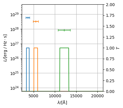
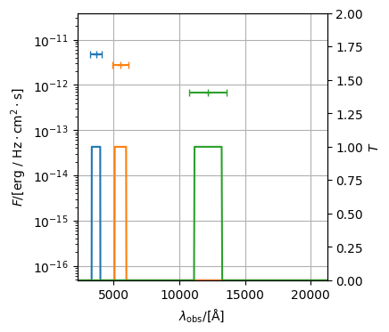
In addition to printing a table of photometry we can also visualise the photometry alongside their filter curves.

lums.plot_photometry(show=True)
fluxes.plot_photometry(show=True)

(<Figure size 350x500 with 2 Axes>,
 <Axes: xlabel='$\\lambda_\\mathrm{obs}/[\\mathrm{\\AA}]$', ylabel='$F/[\\mathrm{\\rm{erg} \\ / \\ \\rm{Hz \\cdot \\rm{cm}^{2} \\cdot \\rm{s}}}]$'>)