The Sed object
This example demonstrates the various methods associated with the Sed class.
Sed objects can be extracted directly from Grid objects or created by Galaxy objects. See tutorials on those objects for more information.
[1]:
import matplotlib.pyplot as plt
import numpy as np
from synthesizer.filters import FilterCollection
from synthesizer.grid import Grid
from synthesizer.igm import Madau96
from synthesizer.sed import Sed, plot_spectra_as_rainbow
from unyt import Angstrom, eV, um
Let’s begin by initialising a grid:
[2]:
grid_dir = "../../tests/test_grid/"
grid_name = "test_grid"
grid = Grid(grid_name, grid_dir=grid_dir)

grid_dir = "../../tests/test_grid/"
grid_name = "test_grid"
grid = Grid(grid_name, grid_dir=grid_dir)
Next, let’s define a target log10age and metallicity and use the built-in Grid method to get the grid point and then extract the spectrum for that grid point.
[3]:
log10age = 6.0  # log10(age/yr)
metallicity = 0.01
spectra_id = "incident"
grid_point = grid.get_grid_point((log10age, metallicity))
sed = grid.get_spectra(grid_point, spectra_id=spectra_id)
sed.lnu *= 1e8  # make the SED bigger
Like other synthesizer objects, we get some basic information about the Sed object by using the print command:
[4]:
print(sed)
----------
SUMMARY OF SED
Number of wavelength points: 9244
Wavelength range: [0.00 Å,             299293000000.00 Å]
log10(Peak luminosity/erg/(Hz*s)):             29.49
log10(Bolometric luminosity/erg/s):36.84609875911521----------
Sed objects contain a wavelength grid and luminosity in the lam and lnu attributes. Both come with units making them easy to convert:
[5]:
print(sed.lam)
print(sed.lnu)
[1.29662e-04 1.33601e-04 1.37660e-04 ... 2.97304e+11 2.98297e+11
 2.99293e+11] Å
[0. 0. 0. ... 0. 0. 0.] erg/(Hz*s)
These also have more descriptive aliases:
[6]:
print(sed.wavelength)
print(sed.luminosity_nu)
[1.29662e-04 1.33601e-04 1.37660e-04 ... 2.97304e+11 2.98297e+11
 2.99293e+11] Å
[0. 0. 0. ... 0. 0. 0.] erg/(Hz*s)
Thus we can easily make a plot:
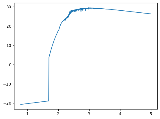
[7]:
plt.plot(np.log10(sed.lam), np.log10(sed.lnu))
plt.show()
/opt/hostedtoolcache/Python/3.10.14/x64/lib/python3.10/site-packages/unyt/array.py:1824: RuntimeWarning: divide by zero encountered in log10
  out_arr = func(np.asarray(inp), out=out_func, **kwargs)
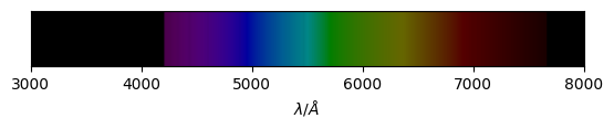
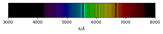
We can also also visualise the spectrum as a rainbow.
[8]:
fig, ax = plot_spectra_as_rainbow(sed)
plt.show()
We can also get the luminosity (\(L\)) or spectral luminosity density per \(\AA\) (\(L_{\lambda}\)):
[9]:
print(sed.luminosity)
print(sed.llam)
[0. 0. 0. ... 0. 0. 0.] erg/s
[0. 0. 0. ... 0. 0. 0.] erg/(s*Å)
Scaling Seds
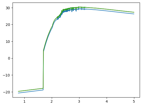
Sed objects can be easily scaled via the * operator. For example,
[10]:
sed3 = sed * 10
sed4 = 10 * sed

plt.plot(np.log10(sed.lam), np.log10(sed.lnu))
plt.plot(np.log10(sed3.lam), np.log10(sed3.lnu))
plt.plot(np.log10(sed4.lam), np.log10(sed4.lnu))
plt.show()
Methods
get_bolometric_luminosity()
This method allows us to calculate the bolometric luminosity of the sed.
[11]:
sed.measure_bolometric_luminosity()
[11]:
unyt_quantity(7.01614828e+44, 'erg/s')
By default any spectra integration will use a trapezoid method. It’s also possible to use the simpson rule.
[12]:
sed.measure_bolometric_luminosity(integration_method="simps")
[12]:
unyt_quantity(6.99398441e+44, 'erg/s')
You can also get the luminosity or lnu in a particular window by passing the wavelengths defining the limits of the window.
[13]:
sed.measure_window_luminosity((1400.0 * Angstrom, 1600.0 * Angstrom))
[13]:
unyt_quantity(4.0480619e+43, 'erg/s')
Notice how units were provided with this window. These are required but also allow you to use an arbitrary unit system.
[14]:
sed.measure_window_luminosity((0.14 * um, 0.16 * um))
[14]:
unyt_quantity(4.0480619e+43, 'erg/s')
[15]:
sed.measure_window_lnu((1400.0 * Angstrom, 1600.0 * Angstrom))
[15]:
unyt_quantity(1.51428832e+29, 'erg/(Hz*s)')
Like the bolometric luminosity there are multiple integration methods that can be used for calculating the window. By default it will use the trapezoid method ("trapz"), but you can also take a simple average.
[16]:
sed.measure_window_lnu(
    (1400.0 * Angstrom, 1600.0 * Angstrom), integration_method="average"
)
[16]:
unyt_quantity(1.5142835e+29, 'erg/(Hz*s)')
Or again use Simpson’s method.
[17]:
sed.measure_window_lnu((1400, 1600) * Angstrom, integration_method="simps")
[17]:
unyt_quantity(1.52094846e+29, 'erg/(Hz*s)')
We can also measure a spectral break by providing two windows, e.g.
[18]:
sed.measure_break((3400, 3600) * Angstrom, (4150, 4250) * Angstrom)
[18]:
np.float64(0.8556966386986625)
There are also a few in-built break methods, e.g. measure_Balmer_break()
[19]:
sed.measure_balmer_break()
[19]:
np.float64(0.8556966386986625)
[20]:
sed.measure_d4000()
[20]:
np.float64(0.9014335946523934)
We can also measure absorption line indices:
[21]:
sed.measure_index(
    (1500, 1600) * Angstrom, (1400, 1500) * Angstrom, (1600, 1700) * Angstrom
)
[21]:
unyt_quantity(5.80884398, 'Å')
We can also measure the UV spectral slope \(\beta\):
[22]:
sed.measure_beta()
[22]:
np.float64(-2.9472901626578625)
By default this uses a single window and fits the spectrum by a power-law. However, we can also specify two windows as below, in which case the luminosity in each window is calcualted and used to infer a slope:
[23]:
sed.measure_beta(window=(1250, 1750, 2250, 2750))
[23]:
np.float64(-2.9533621846623594)
We can also measure ionising photon production rates for a particular ionisation energy:
[24]:
sed.calculate_ionising_photon_production_rate(
    ionisation_energy=13.6 * eV, limit=1000
)
[24]:
unyt_quantity(9.8212605e+54, '1/s')
Observed frame SED
To do this we need to provide a cosmology, using an astropy.cosmology object, a redshift \(z\), and optionally an IGM absorption model.
[25]:
from astropy.cosmology import Planck18 as cosmo

z = 3.0  # redshift
sed.get_fnu(cosmo, z, igm=Madau96)  # generate observed frame spectra
[25]:
unyt_array([0., 0., 0., ..., 0., 0., 0.], 'nJy')
[26]:
plt.plot(np.log10(sed.obslam), np.log10(sed.fnu))
plt.show()
/opt/hostedtoolcache/Python/3.10.14/x64/lib/python3.10/site-packages/unyt/array.py:1824: RuntimeWarning: divide by zero encountered in log10
  out_arr = func(np.asarray(inp), out=out_func, **kwargs)
We can also plot the observed frame spectra as rainbow.
[27]:
fig, ax = plot_spectra_as_rainbow(sed, use_fnu=True)
plt.show()
Photometry
Once we have computed the observed frame SED there is a method on an Sed object that allows us to calculate observed photometry (the same is of course true for rest frame photometry). However, first we need to instantiate a FilterCollection object.
[28]:
filter_codes = [
    f"JWST/NIRCam.{f}"
    for f in [
        "F070W",
        "F090W",
        "F115W",
        "F150W",
        "F200W",
        "F277W",
        "F356W",
        "F444W",
    ]
]  # define a list of filter codes
fc = FilterCollection(filter_codes, new_lam=grid.lam)
[29]:
# Measure observed photometry
fluxes = sed.get_photo_fluxes(fc)
print(fluxes)
------------------------------------------------------------------
|                       PHOTOMETRY (FLUX)                        |
|------------------------------------|---------------------------|
| JWST/NIRCam.F070W (λ = 7.04e+03 Å) | 6.76e-30 erg/(Hz*cm**2*s) |
|------------------------------------|---------------------------|
| JWST/NIRCam.F090W (λ = 9.02e+03 Å) | 5.34e-30 erg/(Hz*cm**2*s) |
|------------------------------------|---------------------------|
| JWST/NIRCam.F115W (λ = 1.15e+04 Å) | 3.86e-30 erg/(Hz*cm**2*s) |
|------------------------------------|---------------------------|
| JWST/NIRCam.F150W (λ = 1.50e+04 Å) | 2.77e-30 erg/(Hz*cm**2*s) |
|------------------------------------|---------------------------|
| JWST/NIRCam.F200W (λ = 1.99e+04 Å) | 1.90e-30 erg/(Hz*cm**2*s) |
|------------------------------------|---------------------------|
| JWST/NIRCam.F277W (λ = 2.76e+04 Å) | 1.10e-30 erg/(Hz*cm**2*s) |
|------------------------------------|---------------------------|
| JWST/NIRCam.F356W (λ = 3.57e+04 Å) | 7.10e-31 erg/(Hz*cm**2*s) |
|------------------------------------|---------------------------|
| JWST/NIRCam.F444W (λ = 4.40e+04 Å) | 4.93e-31 erg/(Hz*cm**2*s) |
------------------------------------------------------------------
Multiple SEDs
The Sed object can actually hold an array of seds and the methods should all work fine.
Let’s create an Sed object with two seds:
[30]:
sed2 = Sed(sed.lam, np.array([sed.lnu, sed.lnu * 2]))
[31]:
sed2.measure_window_lnu((1400, 1600) * Angstrom)
[31]:
unyt_array([1.51428832e+29, 3.02857663e+29], 'erg/(Hz*s)')
[32]:
sed2.measure_window_lnu((1400, 1600) * Angstrom, integration_method="average")
[32]:
unyt_array([1.51428350e+29, 3.02856699e+29], 'erg/(Hz*s)')
[33]:
sed2.measure_beta()
[33]:
array([-2.94729016, -2.94729016])
[34]:
sed2.measure_beta(window=(1250, 1750, 2250, 2750))
[34]:
array([-2.95336218, -2.95336218])
[35]:
sed2.measure_balmer_break()
[35]:
array([0.85569664, 0.85569664])
[36]:
sed2.measure_index(
    (1500, 1600) * Angstrom, (1400, 1500) * Angstrom, (1600, 1700) * Angstrom
)
[36]:
unyt_array([5.80884398, 5.80884398], 'Å')
Combining SEDs
Seds can be combined either via concatenation to produce a single Sed holding multiple spectra from the combined Seds, or by addition to add the spectra contained in two Seds.
To concatenate spectra we can use Sed.concat().
[37]:
print("Shapes before:", sed._lnu.shape, sed2._lnu.shape)
sed3 = sed2.concat(sed)
print("Combined shape:", sed3._lnu.shape)
Shapes before: (9244,) (2, 9244)
Combined shape: (3, 9244)
Sed.concat can take an arbitrary number of Sed objects to combine.
[38]:
sed4 = sed2.concat(sed, sed2, sed3)
print("Combined shape:", sed4._lnu.shape)
Combined shape: (8, 9244)
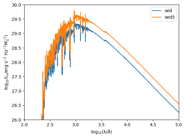
If we want to add the spectra of 2 Sed objects we simply apply the + operator. However, unlike concat, this will only work for Seds with identical shapes.
[39]:
sed5 = sed + sed
plt.plot(np.log10(sed.lam), np.log10(sed.lnu), label="sed")
plt.plot(np.log10(sed5.lam), np.log10(sed5.lnu), label="sed5")
plt.ylim(26, 30)
plt.xlim(2, 5)
plt.xlabel(r"$\rm log_{10}(\lambda/\AA)$")
plt.ylabel(r"$\rm log_{10}(L_{\nu}/erg\ s^{-1}\ Hz^{-1} M_{\odot}^{-1})$")
plt.legend()
plt.show()
plt.close()
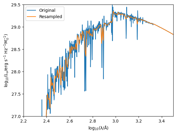
The Sed includes a method to resample an sed, e.g. to lower-resolution or to match observations.
[40]:
sed6 = sed.get_resampled_sed(5)
plt.plot(np.log10(sed.lam), np.log10(sed.lnu), label="Original")
plt.plot(np.log10(sed6.lam), np.log10(sed6.lnu), label="Resampled")
plt.xlim(2.2, 3.5)
plt.ylim(27.0, 29.5)
plt.xlabel(r"$\rm log_{10}(\lambda/\AA)$")
plt.ylabel(r"$\rm log_{10}(L_{\nu}/erg\ s^{-1}\ Hz^{-1} M_{\odot}^{-1})$")
plt.legend()
plt.show()
plt.close()
Spectres: new_wavs contains values outside the range in spec_wavs, new_fluxes and new_errs will be filled with the value set in the 'fill' keyword argument.


Spectres: new_wavs contains values outside the range in spec_wavs, new_fluxes and new_errs will be filled with the value set in the 'fill' keyword argument.
[41]:
print(
    sed.measure_bolometric_luminosity() / sed3.measure_bolometric_luminosity()
)
[1. 0.5 1. ] dimensionless
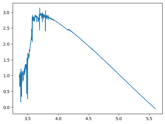
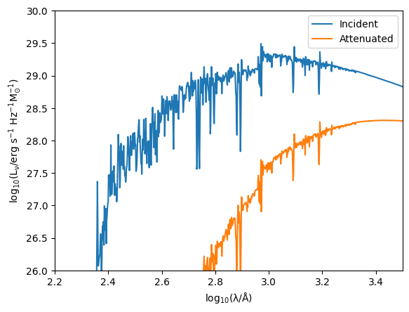
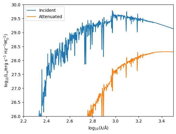
To apply attenuation to an Sed you can use the apply_attenuation method and pass the optical depth. An instance of a dust curve can also be provided but this defaults to a power law with slope = 1 (synthesizer.dust.attenuation.PowerLaw(slope=1)).
[42]:
sed4_att = sed4.apply_attenuation(tau_v=0.7)

plt.plot(np.log10(sed4.lam), np.log10(sed4.lnu[0, :]), label="Incident")
plt.plot(
    np.log10(sed4_att.lam), np.log10(sed4_att.lnu[0, :]), label="Attenuated"
)
plt.xlim(2.2, 3.5)
plt.ylim(26.0, 30.0)
plt.xlabel(r"$\rm log_{10}(\lambda/\AA)$")
plt.ylabel(r"$\rm log_{10}(L_{\nu}/erg\ s^{-1}\ Hz^{-1} M_{\odot}^{-1})$")
plt.legend()
plt.show()
plt.close()
The only other argument apply_attenuation can take is a mask for applying attenuation to speicifc spectra in an Sed with multiple spectra (like an Sed containing the spectra for multiple particles for instance.)
[43]:
sed7_att = sed4.apply_attenuation(
    tau_v=0.7, mask=np.array([1, 0, 0, 0, 0, 0, 0, 0], dtype=bool)
)

plt.plot(np.log10(sed7_att.lam), np.log10(sed4.lnu[1, :]), label="Incident")
plt.plot(
    np.log10(sed7_att.lam), np.log10(sed7_att.lnu[0, :]), label="Attenuated"
)
plt.xlim(2.2, 3.5)
plt.ylim(26.0, 30.0)
plt.xlabel(r"$\rm log_{10}(\lambda/\AA)$")
plt.ylabel(r"$\rm log_{10}(L_{\nu}/erg\ s^{-1}\ Hz^{-1} M_{\odot}^{-1})$")
plt.legend()
plt.show()
plt.close()
If you have an attenuated SED, a natural quantity to calculate is the extinction of that spectra (\(A\)). This can be done either at the wavelengths of the Sed, an arbitrary wavelength/wavelength array, or at commonly used values (1500 and 5500 angstrom) using functions available in the sed module. Note that these functions return the extinction/attenuation in magnitudes. Below is a demonstration.
[44]:
from synthesizer.sed import (
    get_attenuation,
    get_attenuation_at_1500,
    get_attenuation_at_5500,
    get_attenuation_at_lam,
)
from unyt import angstrom, um

# Get an intrinsic spectra
grid_point = grid.get_grid_point((7, 0.01))
int_sed = grid.get_spectra(grid_point, spectra_id="incident")

# Get the attenuated spectra
att_sed = int_sed.apply_attenuation(tau_v=0.7)

# Get attenuation at sed.lam
attenuation = get_attenuation(int_sed, att_sed)
print(attenuation[~np.isnan(attenuation)])

# Get attenuation at 5 microns
att_at_5 = get_attenuation_at_lam(5 * um, int_sed, att_sed)
print(att_at_5)

# Get attenuation at an arbitrary range of wavelengths
att_at_range = get_attenuation_at_lam(
    np.linspace(5000, 10000, 5) * angstrom, int_sed, att_sed
)
print(att_at_range)

# Get attenuation at 1500 angstrom
att_at_1500 = get_attenuation_at_1500(int_sed, att_sed)
print(att_at_1500)

# Get attenuation at 5500 angstrom
att_at_5500 = get_attenuation_at_5500(int_sed, att_sed)
print(att_at_5500)
[       inf        inf        inf ... 0.04221877 0.04207831 0.04193828]
0.08360170415641599
[0.83601817 0.66881427 0.5573455  0.47772428 0.41800898]
2.786725867509981
0.7600168668767144
/opt/hostedtoolcache/Python/3.10.14/x64/lib/python3.10/site-packages/unyt/array.py:1949: RuntimeWarning: invalid value encountered in divide
  out_arr = func(