Emission lines
In addition to creating and manipulating spectral energy distributions, synthesizer can also create Line objects, or more usefully collections of emission lines, LineCollection objects, that can be further analysed or manipulated.
Like spectral energy distributions lines can be extracted directly from Grid objects or generated by Galaxy objects.
Extracting lines from Grid objects
Grids that have been post-processed through CLOUDY also contain information on nebular emission lines. These can be loaded like regular grids, but there are a number of additional methods for working with lines as demonstrated in these examples.
[1]:
import matplotlib.pyplot as plt
import numpy as np
import synthesizer.line_ratios as line_ratios
from synthesizer.grid import Grid
from synthesizer.line import (
    get_diagram_labels,
)
Let’s first introduce the line_ratios module. This contains a set of useful definitions.
[2]:
# the ID of H-alpha
print(line_ratios.Ha)

# the available in-built line ratios ...
print(line_ratios.available_ratios)

# ... and diagrams.
print(line_ratios.available_diagrams)
H 1 6562.80A
('BalmerDecrement', 'N2', 'S2', 'O1', 'R2', 'R3', 'R23', 'O32', 'Ne3O2')
('OHNO', 'BPT-NII')
Next let’s initialise a grid:
[3]:
grid_dir = "../../tests/test_grid"
grid_name = "test_grid"
grid = Grid(grid_name, grid_dir=grid_dir)
We can easily get a list of the available lines:
[4]:
print(grid.available_lines)
['Al 2 1670.79A', 'Ar 3 7135.79A', 'Ar 3 7751.11A', 'Ar 4 2853.66A', 'C 1 1657.91A', 'C 1 1992.01A', 'C 1 2582.90A', 'C 2 1334.53A', 'C 2 1335.66A', 'C 2 1335.71A', 'C 2 2325.40A', 'C 2 2326.93A', 'C 3 1906.68A', 'C 3 1908.73A', 'C 4 1548.19A', 'C 4 1550.77A', 'Ca 2 7291.47A', 'Ca 2 7323.89A', 'Cl 2 8578.70A', 'Fe 2 1.25668m', 'Fe 2 1.27877m', 'Fe 2 1.29427m', 'Fe 2 1.32055m', 'Fe 2 1.32777m', 'Fe 2 1.37181m', 'Fe 2 1.53348m', 'Fe 2 1.59948m', 'Fe 2 1.64355m', 'Fe 2 1.66377m', 'Fe 2 1.67688m', 'Fe 2 1.71113m', 'Fe 2 1.74494m', 'Fe 2 1.79711m', 'Fe 2 1.80002m', 'Fe 2 1.80940m', 'Fe 2 1.89541m', 'Fe 2 1.95361m', 'Fe 2 2395.63A', 'Fe 2 2399.24A', 'Fe 2 2406.66A', 'Fe 2 2410.52A', 'Fe 2 2598.37A', 'Fe 2 2607.09A', 'Fe 2 2611.87A', 'Fe 2 2613.82A', 'Fe 2 2625.67A', 'Fe 2 2628.29A', 'Fe 2 2631.05A', 'Fe 2 2631.32A', 'Fe 2 4243.97A', 'Fe 2 4276.84A', 'Fe 2 4287.39A', 'Fe 2 4319.62A', 'Fe 2 4346.86A', 'Fe 2 4352.79A', 'Fe 2 4358.37A', 'Fe 2 4359.33A', 'Fe 2 4413.78A', 'Fe 2 4416.27A', 'Fe 2 4452.10A', 'Fe 2 4474.90A', 'Fe 2 4814.54A', 'Fe 2 4874.50A', 'Fe 2 4889.62A', 'Fe 2 4905.35A', 'Fe 2 4923.92A', 'Fe 2 4947.39A', 'Fe 2 4973.40A', 'Fe 2 5005.52A', 'Fe 2 5018.44A', 'Fe 2 5020.25A', 'Fe 2 5049.30A', 'Fe 2 5072.41A', 'Fe 2 5111.64A', 'Fe 2 5158.01A', 'Fe 2 5158.79A', 'Fe 2 5169.03A', 'Fe 2 5184.80A', 'Fe 2 5261.63A', 'Fe 2 5273.36A', 'Fe 2 5284.10A', 'Fe 2 5333.66A', 'Fe 2 5376.47A', 'Fe 2 5412.67A', 'Fe 2 5433.15A', 'Fe 2 5527.36A', 'Fe 2 6516.08A', 'Fe 2 7155.17A', 'Fe 2 7172.00A', 'Fe 2 7388.17A', 'Fe 2 7452.56A', 'Fe 2 8616.95A', 'Fe 2 8891.93A', 'Fe 2 9051.95A', 'Fe 2 9226.63A', 'Fe 2 9267.56A', 'Fe 2 9399.04A', 'Fe 2 9470.94A', 'Fe 3 4658.05A', 'Fe 3 4985.87A', 'Fe 3 5270.40A', 'Fe 4 2829.36A', 'Fe 4 2835.74A', 'Fe 4 3094.96A', 'Fe 5 3891.28A', 'Fe 6 3662.50A', 'Fe 6 5176.04A', 'Fe 7 3586.32A', 'Fe 7 3758.92A', 'Fe 7 5720.71A', 'Fe 7 6086.97A', 'H 1 1.00494m', 'H 1 1.09381m', 'H 1 1.28181m', 'H 1 1.87510m', 'H 1 1215.67A', 'H 1 2.16553m', 'H 1 3734.37A', 'H 1 3750.15A', 'H 1 3770.63A', 'H 1 3797.90A', 'H 1 3835.38A', 'H 1 3889.05A', 'H 1 3970.07A', 'H 1 4101.73A', 'H 1 4340.46A', 'H 1 4861.32A', 'H 1 6562.80A', 'H 1 9229.02A', 'H 1 9545.97A', 'He 1 1.08291m', 'He 1 1.08303m', 'He 1 3187.74A', 'He 1 3888.64A', 'He 1 5875.61A', 'He 1 5875.64A', 'He 1 6678.15A', 'He 2 1025.27A', 'He 2 1084.94A', 'He 2 1215.13A', 'He 2 1640.41A', 'He 2 4685.68A', 'Mg 2 2795.53A', 'Mg 2 2802.71A', 'Mg 5 2782.76A', 'Mg 6 1806.00A', 'Mg 7 2628.89A', 'N 2 6548.05A', 'N 2 6583.45A', 'N 3 1749.67A', 'N 4 1486.50A', 'N 5 1238.82A', 'N 5 1242.80A', 'Ne 3 3868.76A', 'Ne 3 3967.47A', 'Ne 4 1601.45A', 'Ne 5 3345.82A', 'Ne 5 3425.88A', 'Ni 2 1.19102m', 'Ni 2 1.93877m', 'Ni 2 6666.80A', 'Ni 2 7377.83A', 'Ni 2 7411.61A', 'O 1 1.12863m', 'O 1 1.12864m', 'O 1 1.12869m', 'O 1 1.12870m', 'O 1 1.12873m', 'O 1 1302.17A', 'O 1 1304.86A', 'O 1 1306.03A', 'O 1 1641.31A', 'O 1 6300.30A', 'O 1 6363.78A', 'O 1 8446.25A', 'O 1 8446.36A', 'O 1 8446.76A', 'O 2 3726.03A', 'O 2 3728.81A', 'O 3 1660.81A', 'O 3 1666.15A', 'O 3 2320.95A', 'O 3 4363.21A', 'O 3 4958.91A', 'O 3 5006.84A', 'O 4 1399.78A', 'O 4 1401.16A', 'O 4 1404.81A', 'O 4 1407.38A', 'O 5 1218.34A', 'O 6 1031.91A', 'O 6 1037.61A', 'S 2 1.02867m', 'S 2 1.03205m', 'S 2 1.03364m', 'S 2 4068.60A', 'S 2 4076.35A', 'S 2 6716.44A', 'S 2 6730.82A', 'S 3 9068.62A', 'S 3 9530.62A', 'Si 2 1179.59A', 'Si 2 1260.42A', 'Si 2 1264.74A', 'Si 2 1265.00A', 'Si 2 1526.71A', 'Si 2 1533.43A', 'Si 3 1206.50A', 'Si 3 1882.71A', 'Si 3 1892.03A', 'Si 4 1393.75A', 'Si 4 1402.77A', 'Si 6 1.96247m', 'Si 7 2.48071m', 'Si 7 2146.64A']
This is also reported if we give the grid to the print function:
[5]:
print(grid)
------------------------------
SUMMARY OF GRID
log10age: [ 6.   6.1  6.2  6.3  6.4  6.5  6.6  6.7  6.8  6.9  7.   7.1  7.2  7.3
  7.4  7.5  7.6  7.7  7.8  7.9  8.   8.1  8.2  8.3  8.4  8.5  8.6  8.7
  8.8  8.9  9.   9.1  9.2  9.3  9.4  9.5  9.6  9.7  9.8  9.9 10.  10.1
 10.2 10.3 10.4 10.5 10.6 10.7 10.8 10.9 11. ]
metallicity: [1.0e-05 1.0e-04 1.0e-03 2.0e-03 3.0e-03 4.0e-03 6.0e-03 8.0e-03 1.0e-02
 1.4e-02 2.0e-02 3.0e-02 4.0e-02]
CMB: None
T_floor: 100
abundance_scalings_carbon: GalacticConcordance
abundance_scalings_nitrogen: GalacticConcordance
alpha: 0.0
axes: ['log10age' 'metallicity']
axes_alternative: ['log10ages' 'metallicities']
cloudy_version: c23.01
constant_density: True
cosmic_rays: True
depletion_model: Jenkins2009_Gunasekera2021
depletion_scale: 0.5
geometry: spherical
grains: Orion
hydrogen_density: 1000.0
incident_axes: ['log10age' 'metallicity']
ionisation_parameter_model: ref
iterate_to_convergence: True
log10age: [ 6.   6.1  6.2  6.3  6.4  6.5  6.6  6.7  6.8  6.9  7.   7.1  7.2  7.3
  7.4  7.5  7.6  7.7  7.8  7.9  8.   8.1  8.2  8.3  8.4  8.5  8.6  8.7
  8.8  8.9  9.   9.1  9.2  9.3  9.4  9.5  9.6  9.7  9.8  9.9 10.  10.1
 10.2 10.3 10.4 10.5 10.6 10.7 10.8 10.9 11. ]
metallicity: [1.0e-05 1.0e-04 1.0e-03 2.0e-03 3.0e-03 4.0e-03 6.0e-03 8.0e-03 1.0e-02
 1.4e-02 2.0e-02 3.0e-02 4.0e-02]
output_cont: True
output_linelist: linelist-standard.dat
parameter_file: c23.01-sps
radius: 0.01
reference_abundance: GalacticConcordance
reference_ionisation_parameter: 0.01
reference_log10age: 6.0
reference_log10age_index: 0
reference_metallicity: 0.01
reference_metallicity_index: 8
resolution: 1.0
stop_T: 500
stop_efrac: -2
turbulence: 100
z: 0.0
available lines: ['Al 2 1670.79A', 'Ar 3 7135.79A', 'Ar 3 7751.11A', 'Ar 4 2853.66A', 'C 1 1657.91A', 'C 1 1992.01A', 'C 1 2582.90A', 'C 2 1334.53A', 'C 2 1335.66A', 'C 2 1335.71A', 'C 2 2325.40A', 'C 2 2326.93A', 'C 3 1906.68A', 'C 3 1908.73A', 'C 4 1548.19A', 'C 4 1550.77A', 'Ca 2 7291.47A', 'Ca 2 7323.89A', 'Cl 2 8578.70A', 'Fe 2 1.25668m', 'Fe 2 1.27877m', 'Fe 2 1.29427m', 'Fe 2 1.32055m', 'Fe 2 1.32777m', 'Fe 2 1.37181m', 'Fe 2 1.53348m', 'Fe 2 1.59948m', 'Fe 2 1.64355m', 'Fe 2 1.66377m', 'Fe 2 1.67688m', 'Fe 2 1.71113m', 'Fe 2 1.74494m', 'Fe 2 1.79711m', 'Fe 2 1.80002m', 'Fe 2 1.80940m', 'Fe 2 1.89541m', 'Fe 2 1.95361m', 'Fe 2 2395.63A', 'Fe 2 2399.24A', 'Fe 2 2406.66A', 'Fe 2 2410.52A', 'Fe 2 2598.37A', 'Fe 2 2607.09A', 'Fe 2 2611.87A', 'Fe 2 2613.82A', 'Fe 2 2625.67A', 'Fe 2 2628.29A', 'Fe 2 2631.05A', 'Fe 2 2631.32A', 'Fe 2 4243.97A', 'Fe 2 4276.84A', 'Fe 2 4287.39A', 'Fe 2 4319.62A', 'Fe 2 4346.86A', 'Fe 2 4352.79A', 'Fe 2 4358.37A', 'Fe 2 4359.33A', 'Fe 2 4413.78A', 'Fe 2 4416.27A', 'Fe 2 4452.10A', 'Fe 2 4474.90A', 'Fe 2 4814.54A', 'Fe 2 4874.50A', 'Fe 2 4889.62A', 'Fe 2 4905.35A', 'Fe 2 4923.92A', 'Fe 2 4947.39A', 'Fe 2 4973.40A', 'Fe 2 5005.52A', 'Fe 2 5018.44A', 'Fe 2 5020.25A', 'Fe 2 5049.30A', 'Fe 2 5072.41A', 'Fe 2 5111.64A', 'Fe 2 5158.01A', 'Fe 2 5158.79A', 'Fe 2 5169.03A', 'Fe 2 5184.80A', 'Fe 2 5261.63A', 'Fe 2 5273.36A', 'Fe 2 5284.10A', 'Fe 2 5333.66A', 'Fe 2 5376.47A', 'Fe 2 5412.67A', 'Fe 2 5433.15A', 'Fe 2 5527.36A', 'Fe 2 6516.08A', 'Fe 2 7155.17A', 'Fe 2 7172.00A', 'Fe 2 7388.17A', 'Fe 2 7452.56A', 'Fe 2 8616.95A', 'Fe 2 8891.93A', 'Fe 2 9051.95A', 'Fe 2 9226.63A', 'Fe 2 9267.56A', 'Fe 2 9399.04A', 'Fe 2 9470.94A', 'Fe 3 4658.05A', 'Fe 3 4985.87A', 'Fe 3 5270.40A', 'Fe 4 2829.36A', 'Fe 4 2835.74A', 'Fe 4 3094.96A', 'Fe 5 3891.28A', 'Fe 6 3662.50A', 'Fe 6 5176.04A', 'Fe 7 3586.32A', 'Fe 7 3758.92A', 'Fe 7 5720.71A', 'Fe 7 6086.97A', 'H 1 1.00494m', 'H 1 1.09381m', 'H 1 1.28181m', 'H 1 1.87510m', 'H 1 1215.67A', 'H 1 2.16553m', 'H 1 3734.37A', 'H 1 3750.15A', 'H 1 3770.63A', 'H 1 3797.90A', 'H 1 3835.38A', 'H 1 3889.05A', 'H 1 3970.07A', 'H 1 4101.73A', 'H 1 4340.46A', 'H 1 4861.32A', 'H 1 6562.80A', 'H 1 9229.02A', 'H 1 9545.97A', 'He 1 1.08291m', 'He 1 1.08303m', 'He 1 3187.74A', 'He 1 3888.64A', 'He 1 5875.61A', 'He 1 5875.64A', 'He 1 6678.15A', 'He 2 1025.27A', 'He 2 1084.94A', 'He 2 1215.13A', 'He 2 1640.41A', 'He 2 4685.68A', 'Mg 2 2795.53A', 'Mg 2 2802.71A', 'Mg 5 2782.76A', 'Mg 6 1806.00A', 'Mg 7 2628.89A', 'N 2 6548.05A', 'N 2 6583.45A', 'N 3 1749.67A', 'N 4 1486.50A', 'N 5 1238.82A', 'N 5 1242.80A', 'Ne 3 3868.76A', 'Ne 3 3967.47A', 'Ne 4 1601.45A', 'Ne 5 3345.82A', 'Ne 5 3425.88A', 'Ni 2 1.19102m', 'Ni 2 1.93877m', 'Ni 2 6666.80A', 'Ni 2 7377.83A', 'Ni 2 7411.61A', 'O 1 1.12863m', 'O 1 1.12864m', 'O 1 1.12869m', 'O 1 1.12870m', 'O 1 1.12873m', 'O 1 1302.17A', 'O 1 1304.86A', 'O 1 1306.03A', 'O 1 1641.31A', 'O 1 6300.30A', 'O 1 6363.78A', 'O 1 8446.25A', 'O 1 8446.36A', 'O 1 8446.76A', 'O 2 3726.03A', 'O 2 3728.81A', 'O 3 1660.81A', 'O 3 1666.15A', 'O 3 2320.95A', 'O 3 4363.21A', 'O 3 4958.91A', 'O 3 5006.84A', 'O 4 1399.78A', 'O 4 1401.16A', 'O 4 1404.81A', 'O 4 1407.38A', 'O 5 1218.34A', 'O 6 1031.91A', 'O 6 1037.61A', 'S 2 1.02867m', 'S 2 1.03205m', 'S 2 1.03364m', 'S 2 4068.60A', 'S 2 4076.35A', 'S 2 6716.44A', 'S 2 6730.82A', 'S 3 9068.62A', 'S 3 9530.62A', 'Si 2 1179.59A', 'Si 2 1260.42A', 'Si 2 1264.74A', 'Si 2 1265.00A', 'Si 2 1526.71A', 'Si 2 1533.43A', 'Si 3 1206.50A', 'Si 3 1882.71A', 'Si 3 1892.03A', 'Si 4 1393.75A', 'Si 4 1402.77A', 'Si 6 1.96247m', 'Si 7 2.48071m', 'Si 7 2146.64A']
available spectra: ['incident', 'linecont', 'nebular', 'transmitted', 'total', 'nebular_continuum']
------------------------------
Let’s choose an age and metallicity we want to get predictions. The in-built method will find the nearest grid point:
[6]:
log10age = 6.0  # log10(age/yr)
metallicity = 0.01
# find nearest grid point
grid_point = grid.get_grid_point((log10age, metallicity))
Let’s get information on a single line, in this case H-beta:
[7]:
line_id = line_ratios.Hb
line = grid.get_line(grid_point, line_id)
print(line)
----------
SUMMARY OF H 1 4861.32A
wavelength: 4861.3 Å
Npart: 1
<log10(luminosity/erg/s)>: 34.52
<equivalent width>: 450 Å
----------
/home/runner/work/synthesizer/synthesizer/src/synthesizer/grid.py:712: FutureWarning: Line objects should be created with a string id, not a list or tuple. This will be removed in a future version.
  Line(
We can do this for a combination of lines (e.g. a doublet) like this. Note: this sums the contribution of each line. If you want separate lines using the get_lines method described below.
[8]:
line = grid.get_line(
    grid_point, [line_ratios.Hb, line_ratios.O3r, line_ratios.O3b]
)
print(line)
----------
SUMMARY OF H 1 4861.32A, O 3 5006.84A, O 3 4958.91A, H 1 4861.32A, O 3 5006.84A, O 3 4958.91A, H 1 4861.32A, O 3 5006.84A, O 3 4958.91A
wavelength: 4942.4 Å
Npart: 1
<log10(luminosity/erg/s)>: 35.47
<equivalent width>: 1359 Å
----------
We can also create a LineCollection a collection of lines which have methods for calculating ratios and diagrams. By default this will create a collection for all available lines but you can also specify which lines you want.
[9]:
lines = grid.get_lines(grid_point)
print(lines)
----------
LINE COLLECTION
number of lines: 215
lines: ['He 2 1025.27A' 'O 6 1031.91A' 'O 6 1037.61A' 'He 2 1084.94A'
 'Si 2 1179.59A' 'Si 3 1206.50A' 'He 2 1215.13A' 'H 1 1215.67A'
 'O 5 1218.34A' 'N 5 1238.82A' 'N 5 1242.80A' 'Si 2 1260.42A'
 'Si 2 1264.74A' 'Si 2 1265.00A' 'O 1 1302.17A' 'O 1 1304.86A'
 'O 1 1306.03A' 'C 2 1334.53A' 'C 2 1335.66A' 'C 2 1335.71A'
 'Si 4 1393.75A' 'O 4 1399.78A' 'O 4 1401.16A' 'Si 4 1402.77A'
 'O 4 1404.81A' 'O 4 1407.38A' 'N 4 1486.50A' 'Si 2 1526.71A'
 'Si 2 1533.43A' 'C 4 1548.19A' 'C 4 1550.77A' 'Ne 4 1601.45A'
 'He 2 1640.41A' 'O 1 1641.31A' 'C 1 1657.91A' 'O 3 1660.81A'
 'O 3 1666.15A' 'Al 2 1670.79A' 'N 3 1749.67A' 'Mg 6 1806.00A'
 'Si 3 1882.71A' 'Si 3 1892.03A' 'C 3 1906.68A' 'C 3 1908.73A'
 'C 1 1992.01A' 'Si 7 2146.64A' 'O 3 2320.95A' 'C 2 2325.40A'
 'C 2 2326.93A' 'Fe 2 2395.63A' 'Fe 2 2399.24A' 'Fe 2 2406.66A'
 'Fe 2 2410.52A' 'C 1 2582.90A' 'Fe 2 2598.37A' 'Fe 2 2607.09A'
 'Fe 2 2611.87A' 'Fe 2 2613.82A' 'Fe 2 2625.67A' 'Fe 2 2628.29A'
 'Mg 7 2628.89A' 'Fe 2 2631.05A' 'Fe 2 2631.32A' 'Mg 5 2782.76A'
 'Mg 2 2795.53A' 'Mg 2 2802.71A' 'Fe 4 2829.36A' 'Fe 4 2835.74A'
 'Ar 4 2853.66A' 'Fe 4 3094.96A' 'He 1 3187.74A' 'Ne 5 3345.82A'
 'Ne 5 3425.88A' 'Fe 7 3586.32A' 'Fe 6 3662.50A' 'O 2 3726.03A'
 'O 2 3728.81A' 'H 1 3734.37A' 'H 1 3750.15A' 'Fe 7 3758.92A'
 'H 1 3770.63A' 'H 1 3797.90A' 'H 1 3835.38A' 'Ne 3 3868.76A'
 'He 1 3888.64A' 'H 1 3889.05A' 'Fe 5 3891.28A' 'Ne 3 3967.47A'
 'H 1 3970.07A' 'S 2 4068.60A' 'S 2 4076.35A' 'H 1 4101.73A'
 'Fe 2 4243.97A' 'Fe 2 4276.84A' 'Fe 2 4287.39A' 'Fe 2 4319.62A'
 'H 1 4340.46A' 'Fe 2 4346.86A' 'Fe 2 4352.79A' 'Fe 2 4358.37A'
 'Fe 2 4359.33A' 'O 3 4363.21A' 'Fe 2 4413.78A' 'Fe 2 4416.27A'
 'Fe 2 4452.10A' 'Fe 2 4474.90A' 'Fe 3 4658.05A' 'He 2 4685.68A'
 'Fe 2 4814.54A' 'H 1 4861.32A' 'Fe 2 4874.50A' 'Fe 2 4889.62A'
 'Fe 2 4905.35A' 'Fe 2 4923.92A' 'Fe 2 4947.39A' 'O 3 4958.91A'
 'Fe 2 4973.40A' 'Fe 3 4985.87A' 'Fe 2 5005.52A' 'O 3 5006.84A'
 'Fe 2 5018.44A' 'Fe 2 5020.25A' 'Fe 2 5049.30A' 'Fe 2 5072.41A'
 'Fe 2 5111.64A' 'Fe 2 5158.01A' 'Fe 2 5158.79A' 'Fe 2 5169.03A'
 'Fe 6 5176.04A' 'Fe 2 5184.80A' 'Fe 2 5261.63A' 'Fe 3 5270.40A'
 'Fe 2 5273.36A' 'Fe 2 5284.10A' 'Fe 2 5333.66A' 'Fe 2 5376.47A'
 'Fe 2 5412.67A' 'Fe 2 5433.15A' 'Fe 2 5527.36A' 'Fe 7 5720.71A'
 'He 1 5875.61A' 'He 1 5875.64A' 'Fe 7 6086.97A' 'O 1 6300.30A'
 'O 1 6363.78A' 'Fe 2 6516.08A' 'N 2 6548.05A' 'H 1 6562.80A'
 'N 2 6583.45A' 'Ni 2 6666.80A' 'He 1 6678.15A' 'S 2 6716.44A'
 'S 2 6730.82A' 'Ar 3 7135.79A' 'Fe 2 7155.17A' 'Fe 2 7172.00A'
 'Ca 2 7291.47A' 'Ca 2 7323.89A' 'Ni 2 7377.83A' 'Fe 2 7388.17A'
 'Ni 2 7411.61A' 'Fe 2 7452.56A' 'Ar 3 7751.11A' 'O 1 8446.25A'
 'O 1 8446.36A' 'O 1 8446.76A' 'Cl 2 8578.70A' 'Fe 2 8616.95A'
 'Fe 2 8891.93A' 'Fe 2 9051.95A' 'S 3 9068.62A' 'Fe 2 9226.63A'
 'H 1 9229.02A' 'Fe 2 9267.56A' 'Fe 2 9399.04A' 'Fe 2 9470.94A'
 'S 3 9530.62A' 'H 1 9545.97A' 'H 1 1.00494m' 'S 2 1.02867m'
 'S 2 1.03205m' 'S 2 1.03364m' 'He 1 1.08291m' 'He 1 1.08303m'
 'H 1 1.09381m' 'O 1 1.12863m' 'O 1 1.12864m' 'O 1 1.12869m'
 'O 1 1.12870m' 'O 1 1.12873m' 'Ni 2 1.19102m' 'Fe 2 1.25668m'
 'Fe 2 1.27877m' 'H 1 1.28181m' 'Fe 2 1.29427m' 'Fe 2 1.32055m'
 'Fe 2 1.32777m' 'Fe 2 1.37181m' 'Fe 2 1.53348m' 'Fe 2 1.59948m'
 'Fe 2 1.64355m' 'Fe 2 1.66377m' 'Fe 2 1.67688m' 'Fe 2 1.71113m'
 'Fe 2 1.74494m' 'Fe 2 1.79711m' 'Fe 2 1.80002m' 'Fe 2 1.80940m'
 'H 1 1.87510m' 'Fe 2 1.89541m' 'Ni 2 1.93877m' 'Fe 2 1.95361m'
 'Si 6 1.96247m' 'H 1 2.16553m' 'Si 7 2.48071m']
available ratios: ['BalmerDecrement', 'N2', 'S2', 'O1', 'R2', 'R3', 'R23', 'O32', 'Ne3O2']
available diagrams: ['OHNO', 'BPT-NII']
----------
We can measure some predifined line ratios:
[10]:
ratio_id = "BalmerDecrement"
ratio = lines.get_ratio(ratio_id)
print(f"{ratio_id}: {ratio:.2f}")
BalmerDecrement: 2.92
Or loop over all pre-defined ratios:
[11]:
for ratio_id in lines.available_ratios:
    ratio = lines.get_ratio(ratio_id)
    print(f"{ratio_id}: {ratio:.2f}")
BalmerDecrement: 2.92
N2: 0.08
S2: 0.06
O1: 0.01
R2: 0.97
R3: 5.97
R23: 9.77
O32: 6.13
Ne3O2: 0.48
We can also easily measure the ratio of an arbitrary set of lines:
[12]:
lines.get_ratio(["Ne 4 1601.45A", "He 2 1640.41A"])
[12]:
np.float64(5.338282707249885e-05)
[13]:
lines.get_ratio(["Ne 4 1601.45A, He 2 1640.41A", "O 3 1660.81A"])
[13]:
np.float64(0.23419729663272387)
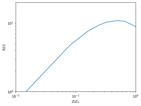
We can plot a ratio against metallicity by looping over the metallicity grid:
[14]:
ratio_id = "R23"
ia = 0  # 1 Myr old for test grid
ratios = []
for iZ, Z in enumerate(grid.metallicity):
    grid_point = (ia, iZ)
    lines = grid.get_lines(grid_point)
    ratios.append(lines.get_ratio(ratio_id))

Zsun = grid.metallicity / 0.0124
plt.plot(Zsun, ratios)
plt.xlim([0.01, 1])
plt.ylim([1, 20])
plt.xscale("log")
plt.yscale("log")
plt.xlabel(r"$Z/Z_{\odot}$")
plt.ylabel(rf"{ratio_id}")
# plt.ylabel(rf'${get_ratio_label(ratio_id)}$')
plt.show()
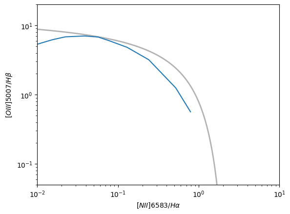
We can also generate “diagrams” pairs of line ratios like the BPT diagram.
The line_ratios also contains some hardcoded literature dividing lines (e.g. Kewley / Kauffmann) that we can use.
[15]:
diagram_id = "BPT-NII"
ia = 0  # 1 Myr old for test grid
x = []
y = []
for iZ, Z in enumerate(grid.metallicity):
    grid_point = (ia, iZ)
    lines = grid.get_lines(grid_point)
    x_, y_ = lines.get_diagram(diagram_id)
    x.append(x_)
    y.append(y_)


# plot the Kewley SF/AGN dividing line

logNII_Ha = np.arange(-2.0, 1.0, 0.01)
logOIII_Hb = line_ratios.get_bpt_kewley01(logNII_Ha)
plt.plot(10**logNII_Ha, 10**logOIII_Hb, c="k", lw="2", alpha=0.3)

plt.plot(x, y)
plt.xlim([0.01, 10])
plt.ylim([0.05, 20])
plt.xscale("log")
plt.yscale("log")

# grab x and y labels, this time use "fancy" label ids
xlabel, ylabel = get_diagram_labels(diagram_id)

plt.xlabel(rf"${xlabel}$")
plt.ylabel(rf"${ylabel}$")
plt.show()
/tmp/ipykernel_4583/636213194.py:17: RuntimeWarning: overflow encountered in power
  plt.plot(10**logNII_Ha, 10**logOIII_Hb, c="k", lw="2", alpha=0.3)
Lines from Galaxy objects
Of course, you’re mainly going to want to generate lines from components of a Galaxy (i.e. parametric or particle based stars or black holes). To do this you can utlise a component’s get_line_intrinsic (intrinsic line emission), get_line_screen (line emission with a simple dust screen) or get_line_attenuated (line emission with more complex dust emission split into a nebular and ISM component) methods. These methods are analogous to those on a grid with the extra component
specific processes, i.e. they return a LineCollection containing the requested lines which can either be singular, doublets, triplets or more.
[16]:
from synthesizer.parametric import SFH, Stars, ZDist
from unyt import Myr

# Make a parametric galaxy
stellar_mass = 10**12
sfh = SFH.Constant(duration=100 * Myr)
metal_dist = ZDist.Normal(mean=0.01, sigma=0.05)
stars = Stars(
    grid.log10age,
    grid.metallicity,
    sf_hist=sfh,
    metal_dist=metal_dist,
    initial_mass=stellar_mass,
)

lc_intrinsic = stars.get_line_intrinsic(grid, line_ids="O 3 4363.21A")
print(lc_intrinsic)
lc_screen = stars.get_line_screen(
    grid, line_ids=("H 1 4340.46A, O 3 4958.91A", "O 3 5006.84A"), tau_v=0.5
)
print(lc_screen)
lc_att = stars.get_line_attenuated(
    grid,
    line_ids=["Ne 4 1601.45A", "He 2 1640.41A", "O 3 5006.84A"],
    tau_v_nebular=0.7,
    tau_v_stellar=0.5,
)
print(lc_att)
----------
LINE COLLECTION
number of lines: 1
lines: ['O 3 4363.21A']
available ratios: []
available diagrams: []
----------
----------
LINE COLLECTION
number of lines: 2
lines: ['H 1 4340.46A, O 3 4958.91A' 'O 3 5006.84A']
available ratios: []
available diagrams: []
----------
----------
LINE COLLECTION
number of lines: 3
lines: ['Ne 4 1601.45A' 'He 2 1640.41A' 'O 3 5006.84A']
available ratios: []
available diagrams: []
----------
In the case of a particle based galaxy you can either get the integrated line emission…
[17]:
from synthesizer.load_data.load_camels import load_CAMELS_IllustrisTNG

# Get the stars from a particle based galaxy
stars = load_CAMELS_IllustrisTNG(
    "../../tests/data/",
    snap_name="camels_snap.hdf5",
    fof_name="camels_subhalo.hdf5",
    physical=True,
)[0].stars

lc_intrinsic = stars.get_line_intrinsic(grid, line_ids="O 3 4363.21A")
print(lc_intrinsic)
lc_screen = stars.get_line_screen(
    grid, line_ids=("H 1 4340.46A, O 3 4958.91A", "O 3 5006.84A"), tau_v=0.5
)
print(lc_screen)
lc_att = stars.get_line_attenuated(
    grid,
    line_ids=["Ne 4 1601.45A", "He 2 1640.41A", "O 3 5006.84A"],
    tau_v_nebular=0.7,
    tau_v_stellar=0.5,
)
print(lc_att)
----------
LINE COLLECTION
number of lines: 1
lines: ['O 3 4363.21A']
available ratios: []
available diagrams: []
----------
----------
LINE COLLECTION
number of lines: 2
lines: ['H 1 4340.46A, O 3 4958.91A' 'O 3 5006.84A']
available ratios: []
available diagrams: []
----------
----------
LINE COLLECTION
number of lines: 3
lines: ['Ne 4 1601.45A' 'He 2 1640.41A' 'O 3 5006.84A']
available ratios: []
available diagrams: []
----------
/home/runner/work/synthesizer/synthesizer/src/synthesizer/particle/galaxy.py:110: RuntimeWarning: In `load_stars`: one of either `initial_masses`, `ages` or `metallicities` is not provided, setting `stars` object to `None`
  self.load_stars(stars=stars)
/home/runner/work/synthesizer/synthesizer/src/synthesizer/particle/galaxy.py:111: RuntimeWarning: In `load_gas`: one of either `masses` or `metallicities` is not provided, setting `gas` object to `None`
  self.load_gas(gas=gas)
/opt/hostedtoolcache/Python/3.10.14/x64/lib/python3.10/site-packages/unyt/array.py:1949: RuntimeWarning: invalid value encountered in divide
  out_arr = func(
Or per particle line emission.
[18]:
lc_intrinsic = stars.get_particle_line_intrinsic(grid, line_ids="O 3 4363.21A")
print(lc_intrinsic)
lc_screen = stars.get_particle_line_screen(
    grid, line_ids=("H 1 4340.46A, O 3 4958.91A", "O 3 5006.84A"), tau_v=0.5
)
print(lc_screen)
lc_att = stars.get_particle_line_attenuated(
    grid,
    line_ids=["Ne 4 1601.45A", "He 2 1640.41A", "O 3 5006.84A"],
    tau_v_nebular=0.7,
    tau_v_stellar=0.5,
)
print(lc_att)
----------
LINE COLLECTION
number of lines: 1
lines: ['O 3 4363.21A']
available ratios: []
available diagrams: []
----------
----------
LINE COLLECTION
number of lines: 2
lines: ['H 1 4340.46A, O 3 4958.91A' 'O 3 5006.84A']
available ratios: []
available diagrams: []
----------
----------
LINE COLLECTION
number of lines: 3
lines: ['Ne 4 1601.45A' 'He 2 1640.41A' 'O 3 5006.84A']
available ratios: []
available diagrams: []
----------